This spring semester I am co-teaching a first-year undergraduate course in computer science at Rice University. The name of the course is COMP 182: Algorithmic Thinking. In reality the name of the course can be somewhat misleading, as I would rather title it “Introduction to Discrete Mathematics and Algorithm Design and Analysis”, but it doesn’t quite roll off the tongue as easily. However, this is not a post about the course or teaching experience, this is a post about one of the upcoming topics in the class: counting.
Introduction
What is counting? In general in discrete mathematics counting concerns deriving mathematical expressions which capture the total number of certain objects that exist. Of course, since we can always make an identical copy of an object and thus increase the count by one, what we really mean is counting the objects up to an appropriate notion of isomorphism, or put plainly, counting distinct objects up to whatever notion of being distinct we choose.
While deriving expressions that capture the counts of objects is an important task, what I want to talk about today goes one step beyond the basics of counting, and is rather aimed to provide you with some applied tools you can sue in the future (of course, in the spirit of Alexander Razborov, here by applied I mean applied to the study of mathematics). However, in order to make this primer relatively complete we will start with some basic results in counting, and then switch to the applications of counting techniques and ideas to more interesting problems.
Permutations
This is the classic problem with which most counting modules of discrete math books start: Find the number of ways in which n distinct objects can be arranged in a line. Key information here is that we are talking about distinct objects and an arrangement in a line. It is easy to show that the total number of such permutations is . We can do so by observing that given an ordering of n-1 objects we have n places to put the new object in, and this holds for every ordering of n-1 objects. More formally, if we denote the number of permutations of n objects by then we have . Also, while we are here, it is useful to note that there is exactly one way of putting no objects down at all, or in other words .
Now, we can take a look at the number of permutations in a slightly different way. For the sake of brevity we will be denoting the set of n positive integers as . Consider the set of functions , we will call this set . Recall that a function is an assignment of outputs for any given input, such that exactly one output value is assigned to any input value. Thus, we can see that , as for any given input we have n choices of the output value, and since all choices are independent of each other we have a total of functions. A reasonable follow up question, is to ask how many of those functions are bijections. Recall that we call a function a bijection iff for any two distinct input values it produces distinct outputs, and for every possible output value there exists an input value that maps to it via our function. In other words, when we look at bijections are precisely the functions that assign to each input a distinct output s.t. for any pair of we have . Note, that since the functions are from to it follows that such an assignment has to use all possible output values. If we look closer at the structure of such bijection, we can realize that it is essentially a permutation of n distinct objects, since we can think of input values as positions on the line, and outputs as the distinct objects we place in those positions. Hence, it follows that there is bijections in .
What we saw above is the fundamental use of counting in combinatorics, we find a combinatorial object of interest (say bijections on the set of n elements) and we count the number of such objects. Often we will see seemingly unrelated families of objects that result in the same total counts, offering us different combinatorial interpretations of the same formula. Furthermore, once we are able to count the number of objects with a given property (say being a bijection) among the total collection of objects (say functions between two sets of n objects) we can immediately get the probability of an object selected uniformly at random to possess the property of interest. In the case of the bijections above we have that . We will see why such simple observations can be of use a bit later in the post.
Count once, count twice
Whenever we count number of certain objects we can sometimes derive the formula based on different inputs. This fact becomes useful in cases when we want to show equality between two expressions. In other words, if we want to prove that two expression are equal, one way to do so can be expressing the count of a particular combinatorial object in two ways, each corresponding to one of the expressions. A quick simple example of this proof technique is given by the handshake lemma in graph theory. Consider a simple graph . We want to evaluate the sum of degrees of all vertices . In order to do so, we can think of a counting argument. What is a degree of any given vertex? It is exactly the number of edges incident to that vertex. Hence, if we sum degrees of all the vertices in a graph it follows that we are indirectly counting the edges of the graph. However, each edge in a simple graph is incident to exactly two vertices. This means that when we summed our degrees, we actually counted occurrence of each edge exactly twice (once per endpoint). Thus, it follows that . While this result at first might not appear as a counting argument, if you think about it for a bit you can recognize that we essentially counted the number of edges in a graph in two ways, once by considering degrees of vertices and once, by simply counting all edges.
Another common example for double counting comes from the problem of finding the number of subsets of a set with n elements. Specifically, on one hand each subset is determined by whether each element is in or out of it, i.e. for each element in we have two possible choices either it is in the subset (1) or it is not (0), thus the total number of possible subsets is the number of all possible strings of n characters over the alphabet of , which is . On the other hand, each subset has some size k where , and we know that the number of ways to pick k elements from n is . Hence, we can conclude that .
A fun extension of the argument above can give us a way to count a slightly more complicated set of objects. We are now interested in how many subsets of a set of n elements have an even number of elements in them. On one hand we can express this number as the sum of with , while on the other hand we can consider the following argument: take an arbitrary subset of a set with n-1 elements, now there is a unique way to extend it to an even sized subset of an n element set. Namely, if our starting subset has an even number of elements, we have to exclude, i.e. assign value 0, to the last element in the n element set, if the starting subset has an odd number of elements then we need to add the last element to it to make the size even, i.e. we assign the value of 1 to the last element. It follows that for any of the subsets of a n-1 element set, there is a unique extension to an even sized subset of n element set. Hence, we can conclude that , or in other words, exactly half of all subsets have an even number of elements in them. This is a nice confirmation to an intuitive guess we might have had originally, but sadly the argument does not extend for the number of subsets with a multiple of 3 elements in them. Let’s formulate this more general version of the question. Let be the number of subsets of a n element set that have size divisible by k. We have from our previous work the values , and . It would be nice if was simply , but sadly that is not an integer. However, with a little bit of elbow grease and usage of binomial theorem we can show that . I will leave the solution to this problem as an exercise for a curious reader.
To summarize, we just saw how counting the same combinatorial objects from two perspectives can serve us as a proof technique for showing equalities between expressions. Thus, we are starting to explore the field of applications that counting techniques provide us.
It exists! But I can’t show you an example
Recall how in the bijection counting question we brought up the probability of a randomly picked function from to to be a bijection. Besides the classical uses of probabilities, such as analyses of randomized algorithms, we can also wield probability as a tool for showing existence of objects with desirable properties. This technique is called probabilistic method and it was pioneered in combinatorics by Paul Erdős. The premise for the application is quite simple at the first glance, in order to show that an object with a desirable property exists, we will show that the probability that a random element belongs to the set of elements with desirable property , where is picked from out universe is greater than 0.
In order to make this more concrete we will work through an application of this method to a graph theoretic question. Consider a complete graph on n vertices . We will call a tournament an orientation of the complete graph, i.e. for every edge in a complete graph we will pick a direction and replace it with a directed edge or . It is easy to check that the total number of tournaments on n vertices is . Now, we are interested in determining whether for there exists a tournament with vertices that contains at least Hamiltonian cycles.
To start, consider the sample space of all tournaments on n vertices and assume the uniform distribution on it. Now, we want to introduce a random variable that counts the number of Hamiltonian circuits (recall that a random variable is a function from the sample space to some set, in our case we have ) in a tournament. Fix a node and consider some permutation of the remaining nodes in the tournament (we have a total of such permutations), we want to know when there is a Hamiltonian cycle that achieves that permutation. Clearly we need to have a directed edge from every predecessor to its successor in the cycle, hence in total we need n edges to point in the correct direction determined by our permutation. Now, let’s define an indicator random variable which is equal to 1 whenever the Hamiltonian cycle defined by the permutation exists in a tournament. We want to compute . In order to do so, we note that we need exactly n edges to have fixed orientation, and hence it follows that the probability of such an event occurring is (since we can think of flipping a coin for orientation of each edge, it’s up to reader to check that this process indeed results in uniform distribution over tournaments). Now, by construction we have where goes over all possible permutations on vertices. Hence, by the linearity of expectation we have that . Now, using our previous result we can conclude that . Hence, since the expected value is it follows that there exists some tournament that has at least Hamiltonian cycles in it.
While it is a stretch to claim that this result is purely enabled by our ability to count combinatorial objects, a lot of key ingredients to the proof rely on our ability to count. Furthermore, this showcases the power of probabilistic method as a non-constructive proof technique for showing existence. In other words, if we can properly count the number of certain objects, we may have a hope of proving interesting results about existence of objects with certain properties.
Instead of conclusion
Of course this is a cursory and incomplete account of counting techniques and applications in discrete mathematics. We haven’t touched upon some key counting ideas such as the inclusion-exclusion principle nor did we discuss any of the more advanced approaches such as generating functions. Furthermore, my account of probabilistic method was purposely short and lacked some of the proper rigor required. However, my aim here was to showcase some of the fun applications of counting techniques and to kindle the spark of interest in the reader. I am not certain whether I will write a follow up to this post any time soon, but stay tuned in case if I do.
Cheers, and don’t forget to count your chickens both before and after they hatch! 🐣
This was my first time I did a real hike alone. A bit more on that topic later, but I can say for sure that picking a reasonably well traveled and not too long of a route was a big plus. I got to the trailhead via an Uber and after stepping over a low fence I began the hike at approximately 10:15 AM PST.
Now, in general the Frenchman mountain hike trail can be split into four key areas: the first hill, the “false” peak, the saddle, and finally the summit. Getting to the top of the first hill didn’t take me that long, but in terms of the combined cardio stress (breathing and heartbeat) this was the most gruesome part of the hike. I suspect that this was more of a result of not being warm enough when starting, combined with a rather fast pace I picked up. Funny enough a group of about 6 teenagers was getting off of the hill in the meantime, and two of them managed to go down, back up, and back down in the time I made it to the top. Once at the top of the hill I had another fun encounter this time spotting an older man with two chihuahuas by his side on their way down form the hike. As I’ve learned later they made it all the way to the summit.
The hill is a nice spot to watch planes from a nearby US Air Force base do their training maneuvers. I was lucky during my hike and managed to see a good amount of action, and even snap a few shots of the planes.
After the hill the real hike began. Shortly after starting my trek up to the “false” peak, I met a local hiker A, who briefly explained to me the overall layout of the trail. He mentioned that a lot of people give up after reaching the first peak, since all they see ahead is a descent followed by an even longer ascent to the summit. From there onwards we essentially hiked in parallel with me being first to the “false” peak, and him being first to the real summit. I am almost certain that hiking with A in sight made this a way more fun and easier experience that if I was doing it completely alone. Additionally, I think it helped me maintain a relatively steady pace, not going too fast or too slow through any of the points.
From the “false” peak you get a nice panoramic view towards the north, and as one previous hiker put it “soul crushing” view of the way up about to come towards the south.
As expected the way down from the “false” peak was not much easier than the way up. In general, this is the pattern that held for most of the hike. The way up is strenuous, but the way down is where you are much more likely to fall. Which is not that surprising given that it is way easier to fall down, than to fall up.
Next up on the list was the saddle, a relatively flat area between the two peaks. Since saddle is still elevated compared to the ground level of Las Vegas, there is a nice little window from which you can catch a glimpse of the Strip, as well as mount Charleston’s peaks.
Finally both A and I made it to the summit of the Frenchman mountain. The views from the top were quite amazing, albeit it wasn’t the clearest day, so the city and mountains behind it looked a tad blurry. According to A, who lived in Las Vegas for more than 10 years, and hiked up and down Frenchman mountain at least 7 or 8 times, one of the best views from the summit is at night, when the Strip is lit up with all the neon lights. I wish I was able to see that, but my stay in Las Vegas is short, and I do not have appropriate flashlight gear to trek up a mountain at night.
While we were taking a bit of a break at the top, A explained that if you walk along the fence of the AT&T tower at the top and then do some basic scrambling, you get to see the eastward view from the mountain including lake Mead. We decided to get to that side as well, so we proceeded forward. Surprisingly the narrow passage around the fence is not particularly scary, but the scramble, especially as you get to the top of it, can make your knees feel a bit weak, especially if like me you have a moderate fear of heights. However, the views from that point are absolutely worth a slight tremble in the knees.
At that point A and I parted ways, as I began my journey back, and A decided to chill at the top for some amount of time. The road back was reasonably hard, as the loose rock and gravel did not make for the sturdiest surfaces to walk down a slope on, and the sun was picking up. I was lucky that this march turned out to be colder than usual, but according to A being on the mountain after 11 AM towards the end of the March would not be the smartest move. On my way back, I had solid noon to 1 PM sun blasting, so I had to make sure to reapply the sunscreen or else I’d end up being a fine shade of lobster red by the time I’d be back.
While the planes, the views, and the weather were on my side this time, the local fauna was timid. I only managed to spot a few tiny birds (barely above the size of a hummingbird), but decided not to snap any pictures of them, since they essentially blended with the rocks. The vegetation on the mountain was desert-like as expected.
There were also some cool rocks on the way which seemed to burst from within the other rock formations. They were deep amber in color and a few small fragments I picked up felt almost glass like: relatively light, fragile feeling, yet sharp around thinner edges.
However, since my knowledge of geology and mineralogy is nil, I had no way to identify what those veins were. I probably can Google it, but will rather wait until my parents see the pictures and do the mineralogy Google research for me.
At the end of the hike I felt tired, but accomplished. The solo mission was a complete success, and I enjoyed the views and the challenge. On the way back there were a few moments when as far as I could see I was the only person on the trail. Despite part of my mind thinking about how it is not the best idea to chill in the middle of a desert at noon, I still found it quite meditative to stop in more windy places and take in the vast scale of the nature surrounding me.
I would like to claim that due to my amazing balancing skills and a good choice of hiking boots I managed to stay on my feet for the whole hike. However, such a claim would be false. Towards the end of the hike, as I was descending from the “false” peak, I managed to slip and slide on a bunch of gravel and made full contact with ground. It was a minor and rather graceful fall, so I am not expecting more than a minor bruise on my hip and moderate sized bruise on my ego.
Now, after I made it back to the AirBnB, and am enjoying a nice cold beer, I start feeling my legs and feet drafting a complaint about today’s adventure. Hopefully, I will be mostly recovered by tomorrow as ahead lies an approximately 3 hour drive towards the Zion National Park.
In conclusion, I would recommend the Frenchman mountain trail to anyone who enjoys desert mountain hiking and looks for a moderate hike. Main difficulties of this hike are the steep inclines and loose gravel. However, the overall short length of the trail compensates for it making a round trip in 3.5-4 hours more that achievable, even if you stop frequently for pictures.
On October 16th around 6 AM the plane taking me to Baltimore, Maryland took off from the Hobby airport in Houston. I generally do not mind very early morning flights, and since I still retain the magical (and much envied) ability to sleep on the planes the commute was fine. I arrive in BWI around 10 AM and after picking up my luggage headed directly for the Sheraton Inner Harbor hotel. The hotel did not have an early check-in option available, so I dropped off my bags and went for a walk. I found a neat coffee shop and spent a bit of time catching up on some reading.
Inner harbor in Baltimore, Maryland, around 10:45 AM. Not the best shot, but I managed to catch a bird in this one, so I am posting it.Inner harbor in Baltimore, Maryland, still around 10:45 AM. Still not the best shot, but also I didn’t take any particularly good ones this time. I guess being awake since 3 AM ain’t helpful for my artistic eye.Washington monument at Mt. Vernon in Baltimore, Maryland, circa noon. Quality of the shots improves as the day goes on.
After the coffee break, I met up with Evan Mata and we caught up on school life, travel stories, and I finally got my oyster fix. Two key takeaways from our lunch were as follows: (1) we both wish we took more math courses in college (and in fact this appears to be a common trend for many of my college friends), and (2) Maryland oysters are still delicious, albeit not as cheap as I remembered.
The Local Oyster (Mt. Vernon location). Bloody Mary with an oyster and a dozen of fresh oysters. Hence 13 oysters in total for me, quite a lunch in my opinion.
After the lunch I made it back to the hotel where I finally could check in and catch my breath before the opening keynotes for the ASM NGS 2022. Besides the keynotes, and a brief chat over dinner the first day was not jam packed with activities, so I was able to crash early and catch up on some of the sleep that I missed due to the early flight.
Next day I attended a series of the talks in the morning, after which I headed for the University of Maryland, College Park. UMD campus is quite expansive, and in some strange way it reminded me of the University of Tennessee in Knoxville. The computer science building at UMD is quite impressive both in size and design, and many offices tend to have nice floor to ceiling windows, which is an awesome touch. I did not have too much time to explore the campus, as the visit was relatively tightly packed with meetings, and as soon as those were wrapped up I headed back to Baltimore.
E. A. Fernandez IDEA Factory on the University of Maryland College Park campus. The only shot I took at the UMD campus (sadly, since the campus is quite pretty IMHO).
Although, I unfortunately missed most of the afternoon talks on the first day, I still managed to catch the poster session. In general, I am a big fan of poster sessions. The main benefit of a poster (as opposed to a talk) is the ability to ask a multitude of questions about the nitty-gritty details of the work without feeling guilty of encroaching on other people’s time. I found a good number of quite interesting posters relating to SARS-CoV-2, bacteria and horizontal gene transfer, and even a poster on a speed up for neighbor-joining algorithm. After the poster session I briefly caught up with Mike Nute over dinner which importantly included a crab cake (another checklist food item for me on this trip).
Grabbing dinner with Mike Nute at Phillips Seafood in Baltimore, Maryland. Quite solid crab cake and overall good spread of seafood. Very enjoyable dinner option not too far from the conference hotel location.
The crab cake ended up being quite good, although I have a feeling that with a bit of effort I can probably make a comparable if not a better one at home. However, crab meat is not cheap to come by, so I am not likely to test that hypothesis any time in the near future.
Tuesday was a full conference day for me. I attended all of the talks that day, and tried to keep a list of close notes for most of them. Unfortunately the tables at the conference did not have any outlets or power strips connecting to them or running along the floor. Thus, my note taking was cut short towards the second half of the afternoon, as my laptop ran out of its battery.
The last talk session of they day was a wastewater focused mini-symposium. The talks in this session were quite interesting, and indeed reflected a lot of my experiences and concerns when dealign with wastewater data. Namely, issues of the data quality, metadata annotation, and general complexity of the wastewater samples, which in certain cases ends up being overlooked. I was very happy that I was able to give a talk in this session as well. I was presenting the joint work between Treangen and Stadler labs at Rice University in conjunction with the Houston Health Department. My talk focused on QuaID: a software package we developed for sensitive detection of recently emerged SARS-CoV-2 variants in wastewater sequencing data (preprinted at medRxiv).
My first conference talk looked something like this. ASM NGS 2022, Day 2, wastewater session.Some scallops (which were yummy) at the Watershed in Baltimore, Maryland. Post talk dinner feels good, although sitting on a rooftop terrace might not have been the best decision given it was in the low 50 F range?
Overall the talk went very well, and I enjoyed the experience. Of course, as any public performance giving the talk came with a fair deal of stage fright and nervousness. However, extensive practice runs with my labmates, adviser, and collaborators helped a lot in mitigating anxiety, and polishing the presentation content. As per usual, I do think that several moments could have been executed better on my part, but I’ll hope to use that as the knowledge for preparing my next presentations.
The evening continued on into another poster session with a fair number of exciting wastewater and clinical SARS-CoV-2 work, as well as some benchmarking studies of interest. I felt that the second poster session was a tad bit more lively than the first one, but it also could have been an artifact of my post-talk state. After the poster session, I joined a large-ish group of attendees for dinner and chats. Scallops were not on my Baltimore food checklist, but among the seafood options offered at the Watershed they stood out as an interesting choice. Overall I enjoyed them, although next time I will probably go for the crab cakes.
The last day of the conference was relatively short with only a morning session of the talks. There was a plenty of interesting talks this day, and I was quite pleasantly surprised to hear several talks involving deep learning in a principled and well motivated way. The only drawback of this session was the amount of lightning talks given back to back. It was at times hard to properly note down all the details, and due to the format and the fact that this was the last day it was harder to follow up with the presenters to discuss some of the finer details of their work. However, I still managed to take a good amount of notes, and expand my “papers to read” list by a dozen or so manuscripts.
After the conference, I checked out of the hotel and headed to our last stop before the airport: Johns Hopkins University. First we stopped by the medical campus and grabbed a lunch, which consisted of an absolutely wonderful lamb stew with rice. Then we moved to the Homewood campus pictures of which are attached below.
Afghani food at Kabobi in Baltimore, Maryland near JHU Medical Campus. Amazing lamb stew with veggies, a very hearty and comfortable meal.Johns Hopkins University, Homewood campus, Baltimore, Maryland. Autumn gets to be particularly pretty around this time with all the beautiful colors on the trees.
Being on JHU Homewood campus reminded me of one of the greatest pleasures in the fall season: observing the colorful trees in a light cool breeze. However, similarly to the UMD visit, I did not have much time to wander around and observe the trees, as we mainly focused on the scheduled meetings.
At the end of the trip I was absolutely exhausted, but overall happy with the experience. I managed to tick off several of the key food checklist items on this visit. Of course more importantly, I really enjoyed attending the ASM NGS conference, and finally being able to experience an in-person conference. Giving a talk was a huge added benefit, and all the meetings, lunches, and dinners with multiple new and old acquaintances and collaborators (some of whom I finally got to see in person) made this a very memorable trip.
Getting back to Houston late at night I was reminded that this is a spooky season 🎃!
Hi, if you expected a weekly post here I am extremely glad that you are someone who checks out my blog regularly. However, this week I am skipping my regular post. No, I am not traveling nor am I absolutely crushed by 1001 deadlines. In fact, I had a solid post mapped out and even partially written, but I did not have the energy to fully wrap it up in time.
What’s going to happen next?
First, I am going to be traveling mid of October onwards (within the USA), so catch me on tour (not really). Hence, I am likely to have more travel and conference content rather than the “vignettes” style posts. Nevertheless stay tuned as I will try to provide some form of content be it travel updates or micro-posts at least every Monday.
Second, I am seriously debating taking a tropical vacation. I wish it meant going to an actual tropical resort, but rather I mean a cursory exploration of: (a) tropical geometry (via Maclagan and Sturmfels, 2009); (b) algebraic statistics (via Sullivant, 2018) ; and (c) how all of this relates to bioinformatics (via papers + some of the Lior Pachter’s blog posts). I am not perfectly sure this is the journey I am interested in for the next few months, but it is one of the possibilities I am exploring.
Third, I believe that my most recent posts were avoidant of code snippets which is in part justified by the lack of time to write out meaningful code primers. However, this is not the format I am fully enjoying. I believe that code snippets bring the life to abstract concepts and provide an extra layer of interactive experience that can be beneficial in learning process. Hence, I will be making more effort to bring some code to the posts going forward.
As I mentioned in the previous post, I am taking some time off to figure out which direction to pursue next in the blog post series. However, that does not mean that the whole series itself is going into hiatus. In the meantime, I am going to cover a few other topics in phylogenetics. Additionally, I will cross post some of the one-off posts on Dr. Treangen’s lab website. Now, with logistics out of the way let’s get into tree rearrangements.
Introduction
Whenever we are faced with a problem in combinatorial optimization it is often convenient (or even necessary as the majority of interesting problems turn out to be NP-hard) to come up with some heuristic methods. In particular, we often want to explore a “neighborhood” of an object and locate optimal candidates within this neighborhood after which the search can continue from the new local optima. In order to talk about neighborhoods we need to define a metric on the space of objects we are working with (we talked about metric spaces on phylogenetic trees in severalpreviousposts, but in this case we are focusing solely on the tree topology and associated finite metric spaces). In the context of a search problem it is useful to think about the neighborhood of an object as a set of objects that can be obtained from the initial object via some fixed operation. In phylogenetics such operations on trees are typically called tree rearrangements (Felsenstein, 2004). In this post we will take a look at three classical tree rearrangement operations, but keep in mind that there are other ways to mutate trees which lead to different geometries on the tree space.
In the next three sections we will introduce in detail each of the rearrangement operations in the order of increasing neighborhood sizes considered and then briefly discuss the relationships between these three classes, as well as some implications for computational complexity of related problems.
Nearest neighbor interchange
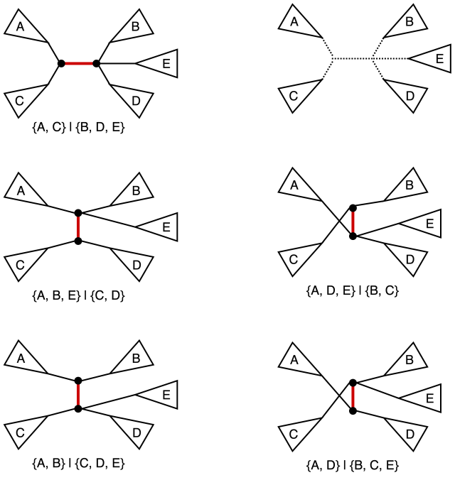
Nearest neighbor interchange (NNI) operation on a tree consists of picking an internal edge (i.e. an edge that is not incident to a leaf) deleting it along with the four edges incident to the vertices of the original edge, after obtaining four components as the result of the deletion there are three distinct ways of reconnecting them back out of which one yields the original tree. It is easy to see that for an unrooted bifurcating tree on n taxa (i.e. a tree with n leaves) there is a total of n-3 internal edges, and hence a total of 2(n-3) NNI-neighbors. We also note that the operation in this classical sense is defined for bifurcating trees (hence the guarantee that the NNI yields for connected components after the edge removal step). The figure below provides an example of NNI and the resulting tree neighbors.
The original tree is shown in the top left corner and the marked edge is the internal edge along which we perform the NNI. The four connected components labeled A, B, C, and D are shown in the top right corner. The resulting two new trees are shown at the bottom. For each of the three trees we also include the split corresponding to the marked edge.
For a small value of n we can reasonably visualize the adjacency structure on the tree space induced by the NNI operation. Namely we can identify non-isomorphic (read: distinct from the point of view of the properties we care about) labeled tree topologies as vertices and let two vertices be connected by an edge iff we can obtain one topology from another via a single NNI.
An example of adjacency graph on the space of 5 taxa unrooted bifurcating trees under the NNI operation. Original figure and caption are taken from Felsenstein, 2004, p. 40.
In general a phylogenetic tree encountered (or I guess inferred) in the wild might not be bifurcating, so it is quite natural to ask how does one generalize the notion of NNI to an arbitrary labeled unrooted tree. At the core of this operation is the process of picking a distinguished edge and then swapping components resulting from an edge deletion operation. Thus, in the case of a multifurcating tree we simply can do the same operation but with a larger set of neighbors being generated. An example is provided in the figure below.
A few possible neighbors of the original multifurcating tree (top left) under the NNI on trees with varying internal node degrees. Note that in the case where we allow multifurcations we ought to be careful in the way we define the NNI operation as some interchanges can be problematic (consider what happens if we reconnect 5 components into a star graph).
There is some amount of work on the NNI operations and NNI induced metric on phylogenetic trees (Hon and Lam, 1999), although the area tends to feel relatively sparse in terms of the research done.
Subtree prune and regraft
Subtree prune and regraft (SPR) operation on a tree consists of snipping off a branch (which can be an internal or external edge) and then inserting the snipped off subtree onto one of the edges of the remaining tree. This operation is quite well illustrated by its name, especially if you ever had to deal with grafts on actual trees (my grandfather loved to experiment with fruit tree grafting, which to his credit managed to give us a wonderful apricot half-tree on a wild apricot that used to grow in the garden). The figure below is an example of a SPR operation performed on a tree.
A subtree is snipped off from the original tree along the edge marked in red (top left) and then re-attached to the remaining tree on an edge marked in orange. It can be helpful to think of this operation as temporarily turning one of the subtrees into a rooted tree and then reinserting its root into the remaining tree.
It is easy to see that SPR operation results in a larger neighborhood set than the NNI operation. It also useful to note that any tree T’ that can be obtained from a tree T via a single NNI can also be obtained via a single SPR. In other words, if we define the set NNI(T) of trees that can be obtained from T via a single NNI, and the set SPR(T) of trees that can be obtained from T via a single SPR, then the following inclusion holds: NNI(T)⊆SPR(T) (Maddison, 1991). In the spirit of ancient geometers instead of a formalized proof, we will provide the following figure and leave it up to the reader to convince themselves that the inclusion above is indeed true.
Similarly to the NNI case we can compute the exact number of neighbors under the SPR operation for an unrooted bifurcating binary tree on n taxa. The size of this neighborhood similarly to the NNI case is independent of the topology of the tree T and is equal to 2(n-3)(2n-7) with a detailed counting argument provided by Allen and Steel, 2001 on p. 4.
We also note that the way in which we graft a subtree back in will always create an internal node of degree 3, so without a modification to this operation the question of generalizing it to multifurcating trees can be ill-posed.
Tree bisection and reconnection
Tree bisection and reconnection (TBR)operation is the most expansive operation among the three we are considering in this post, in the sense that it yields the largest neighborhoods. TBR consists of splitting the original tree T into two subtrees T’ and T” along a branch and then reconnecting them by joining any two branches of T’ and T” via an edge (in case if one of the subtrees is just a leaf the leaf is simply joined back to the tree via a new branch; in all cases vertices might have to be added to maintain a proper bifurcating tree). The figure below illustrates a TBR operation being performed.
The original tree is shown in the upper left corner. The edges to be joined are marked in orange (bottom), and the new joining edge is marked in red (bottom right). Note, that the tree obtained after the specified TBR operation is isomorphic to the tree obtained via SPR with regrafting onto the orange edge of the bottom left subtree.
The inclusion we observed for the NNI and SPR neighborhoods extends further and the following holds: NNI(T)⊆SPR(T)⊆TBR(T) (Maddison, 1991). Furthermore, by noting that any TBR can be thought of as a two step process where we first re-attach T” onto the specified edge of T’ and then reposition the attached T’ in order to get correct edge match, we can show that any TBR operation can be replicated by at most two successive SPR operations.
Finally, we note that unlike NNI and SPR, the TBR neighborhood size does depend on the topology of the tree T. However, and upper bound on the size of the neighborhood can be computed and is given by (2n-3)(n-3)2 (Allen and Steel, 2001, p.5).
Induced metrics and computational (in)tractability
We already noted in the introduction that the tree rearrangement operations induce corresponding metrics on the space of phylogenetic trees (more precisely in our current case: the space of unrooted bifurcating tree topologies). We will denote these metrics dNNI(T, T’), dSPR(T, T’), and dTBR(T, T’), respectively. From the inclusion relation on the neighborhoods it immediately follows that for any two unrooted bifurcating trees we have the following inequality: dTBR(T, T’)≤dSPR(T, T’)≤dNNI(T, T’). Furthermore, from our observation in the previous section we also can conclude that dSPR(T, T’)≤2×dTBR(T, T’).
Although we have provided an explicit example of the adjacency graph under NNI metric for the space of unrooted bifurcating trees on 5 taxa, it is not immediately obvious that in the general case the NNI adjacency graph will be connected (i.e. we are not a priori guaranteed to have a connected metric space). However, it turns out that indeed the adjacency graph under the NNI metric is indeed connected, and hence the metric space induced by dNNI(T, T’) is connected. It is easy to see that as a corollary we also get connectedness for the SPR and TBR spaces.
Since the metric spaces are connected and finite we can ask what are their respective diameters (i.e. the smallest distance between two points furthest apart in the space; this is the same definition as the graph diameter). An interesting non-trivial bound on the diameter of the NNI space was derived by Li et al., 1996: authors show that the diameter of the NNI adjacency graph (which we will denote as ΔNNI) is bounded below and above by nlogn terms. More precisely, the following inequality holds: . Allen and Steel, 2001 extend this result to the SPR and TBR cases giving the following inequalities: (a) n/2-o(n)≤ΔSPR≤n-3; (b) n/4-o(n)≤ΔTBR≤n-3.
However, knowing the diameter of a space does not imply that we can easily compute the distances within it (i.e. shortest paths via NNI, SPR or TBR operations from one tree to another). In fact, the problems of computing NNI, SPR or TBR distance between two arbitrary unrooted bifurcating trees are all NP-hard (NNI: DasGupta et al., 2000; SPR: Bordewich and Semple, 2005, Hickey et al., 2008; TBR: Hein et al., 1996). Allen and Steel, 2001 show that the SPR distance is fixed-parameter tractable, but in general the fixed-parameter tractability results in algorithms that can work efficiently only on small trees or pairs of trees which are relatively close to each other (for a more principled discussion see Whidden and Matsen, 2018). In general, it appears to be a rare case for a metric that is biologically interpretable to be efficiently computable, and vice-a-versa (take for example the Robinson-Foulds distance which is efficiently computable, but not biologically well grounded). There are some recent attempts at developing variants of tree rearrangement operations that have both biological interpretability and are computationally tractable (Collienne and Gavryushkin, 2021).
While we could possibly discuss other tree rearrangement operations or explore the discrete geometries arising from the ones we mentioned in more detail, such work would likely require multiple posts. Thus, we will wrap up here and invite the reader to continue the exploration via following the links provided in the references section.
Data and code availability
All illustrations with the exception of the one from Felsenstein, 2004 were made with draw.io. No additional materials or code were used in this post.
What’s next
I am still deliberating on the exact direction to take for the next stretch of posts, so in the meantime I am intending to continue the one-off posts where I pick a random, but interesting to me, topic in mathematical phylogeny and try to write a coherent text about it. As per usual, if you are interested in me writing about a specific topic do not hesitate to reach out.
References
Allen, Benjamin L., and Mike Steel. “Subtree transfer operations and their induced metrics on evolutionary trees.” Annals of combinatorics 5, no. 1 (2001): 1-15. https://doi.org/10.1007/s00026-001-8006-8
Bordewich, Magnus, and Charles Semple. “On the computational complexity of the rooted subtree prune and regraft distance.” Annals of combinatorics 8, no. 4 (2005): 409-423. https://doi.org/10.1007/s00026-004-0229-z
Collienne, Lena, and Alex Gavryushkin. “Computing nearest neighbour interchange distances between ranked phylogenetic trees.” Journal of Mathematical Biology 82, no. 1 (2021): 1-19. https://doi.org/10.1007/s00285-021-01567-5
Gupta, Bhaskar Das, Xin He, Tao Jiang, Ming Li, and John Tromp. “On computing the nearest neighbor interchange distance.” In Discrete Mathematical Problems with Medical Applications: DIMACS Workshop Discrete Mathematical Problems with Medical Applications, December 8-10, 1999, DIMACS Center, vol. 55, p. 125. American Mathematical Soc., 2000. PDF on author’s page
Hein, Jotun, Tao Jiang, Lusheng Wang, and Kaizhong Zhang. “On the complexity of comparing evolutionary trees.” Discrete Applied Mathematics 71, no. 1-3 (1996): 153-169. https://doi.org/10.1016/S0166-218X(96)00062-5
Hickey, Glenn, Frank Dehne, Andrew Rau-Chaplin, and Christian Blouin. “SPR distance computation for unrooted trees.” Evolutionary Bioinformatics 4 (2008): EBO-S419. https://doi.org/10.4137/EBO.S419
Hon, Wing-Kai, and Tak-Wah Lam. “Approximating the nearest neighbor interchange distance for evolutionary trees with non-uniform degrees.” In International Computing and Combinatorics Conference, pp. 61-70. Springer, Berlin, Heidelberg, 1999. https://doi.org/10.1007/3-540-48686-0_6
Li, Ming, John Tromp, and Louxin Zhang. “On the nearest neighbour interchange distance between evolutionary trees.” Journal of Theoretical Biology 182, no. 4 (1996): 463-467. https://doi.org/10.1006/jtbi.1996.0188
Maddison, David R. “The discovery and importance of multiple islands of most-parsimonious trees.” Systematic Biology 40, no. 3 (1991): 315-328. https://doi.org/10.1093/sysbio/40.3.315
Whidden, Chris, and Frederick A. Matsen. “Calculating the unrooted subtree prune-and-regraft distance.” IEEE/ACM transactions on computational biology and bioinformatics 16, no. 3 (2018): 898-911. https://doi.org/10.1109/TCBB.2018.2802911


![[n]=\{1, 2, 3, ..., n\}](https://s0.wp.com/latex.php?latex=%5Bn%5D%3D%5C%7B1%2C+2%2C+3%2C+...%2C+n%5C%7D&bg=fafafa&fg=6c6c8c&s=0&c=20201002)
![f:[n]\to[n]](https://s0.wp.com/latex.php?latex=f%3A%5Bn%5D%5Cto%5Bn%5D&bg=fafafa&fg=6c6c8c&s=0&c=20201002)
![\mathcal{F}_n=\{f|f:[n]\to[n]\}](https://s0.wp.com/latex.php?latex=%5Cmathcal%7BF%7D_n%3D%5C%7Bf%7Cf%3A%5Bn%5D%5Cto%5Bn%5D%5C%7D&bg=fafafa&fg=6c6c8c&s=0&c=20201002)

![i\in[n]](https://s0.wp.com/latex.php?latex=i%5Cin%5Bn%5D&bg=fafafa&fg=6c6c8c&s=0&c=20201002)


![j\in[n]](https://s0.wp.com/latex.php?latex=j%5Cin%5Bn%5D&bg=fafafa&fg=6c6c8c&s=0&c=20201002)


![[n]](https://s0.wp.com/latex.php?latex=%5Bn%5D&bg=fafafa&fg=6c6c8c&s=0&c=20201002)


![\sigma:[n]\to[n]](https://s0.wp.com/latex.php?latex=%5Csigma%3A%5Bn%5D%5Cto%5Bn%5D&bg=fafafa&fg=6c6c8c&s=0&c=20201002)


![\mathbb{E}[X]=\sum_{\sigma}\mathbb{E}[X_\sigma]=\sum_{\sigma}Pr(X_\sigma =1)](https://s0.wp.com/latex.php?latex=%5Cmathbb%7BE%7D%5BX%5D%3D%5Csum_%7B%5Csigma%7D%5Cmathbb%7BE%7D%5BX_%5Csigma%5D%3D%5Csum_%7B%5Csigma%7DPr%28X_%5Csigma+%3D1%29&bg=fafafa&fg=6c6c8c&s=0&c=20201002)
![\mathbb{E}[X]=(n-1)!/2^n](https://s0.wp.com/latex.php?latex=%5Cmathbb%7BE%7D%5BX%5D%3D%28n-1%29%21%2F2%5En&bg=fafafa&fg=6c6c8c&s=0&c=20201002)


 .
.