This spring semester I am co-teaching a first-year undergraduate course in computer science at Rice University. The name of the course is COMP 182: Algorithmic Thinking. In reality the name of the course can be somewhat misleading, as I would rather title it “Introduction to Discrete Mathematics and Algorithm Design and Analysis”, but it doesn’t quite roll off the tongue as easily. However, this is not a post about the course or teaching experience, this is a post about one of the upcoming topics in the class: counting.
Introduction
What is counting? In general in discrete mathematics counting concerns deriving mathematical expressions which capture the total number of certain objects that exist. Of course, since we can always make an identical copy of an object and thus increase the count by one, what we really mean is counting the objects up to an appropriate notion of isomorphism, or put plainly, counting distinct objects up to whatever notion of being distinct we choose.
While deriving expressions that capture the counts of objects is an important task, what I want to talk about today goes one step beyond the basics of counting, and is rather aimed to provide you with some applied tools you can sue in the future (of course, in the spirit of Alexander Razborov, here by applied I mean applied to the study of mathematics). However, in order to make this primer relatively complete we will start with some basic results in counting, and then switch to the applications of counting techniques and ideas to more interesting problems.
Permutations
This is the classic problem with which most counting modules of discrete math books start: Find the number of ways in which n distinct objects can be arranged in a line. Key information here is that we are talking about distinct objects and an arrangement in a line. It is easy to show that the total number of such permutations is . We can do so by observing that given an ordering of n-1 objects we have n places to put the new object in, and this holds for every ordering of n-1 objects. More formally, if we denote the number of permutations of n objects by then we have . Also, while we are here, it is useful to note that there is exactly one way of putting no objects down at all, or in other words .
Now, we can take a look at the number of permutations in a slightly different way. For the sake of brevity we will be denoting the set of n positive integers as . Consider the set of functions , we will call this set . Recall that a function is an assignment of outputs for any given input, such that exactly one output value is assigned to any input value. Thus, we can see that , as for any given input we have n choices of the output value, and since all choices are independent of each other we have a total of functions. A reasonable follow up question, is to ask how many of those functions are bijections. Recall that we call a function a bijection iff for any two distinct input values it produces distinct outputs, and for every possible output value there exists an input value that maps to it via our function. In other words, when we look at bijections are precisely the functions that assign to each input a distinct output s.t. for any pair of we have . Note, that since the functions are from to it follows that such an assignment has to use all possible output values. If we look closer at the structure of such bijection, we can realize that it is essentially a permutation of n distinct objects, since we can think of input values as positions on the line, and outputs as the distinct objects we place in those positions. Hence, it follows that there is bijections in .
What we saw above is the fundamental use of counting in combinatorics, we find a combinatorial object of interest (say bijections on the set of n elements) and we count the number of such objects. Often we will see seemingly unrelated families of objects that result in the same total counts, offering us different combinatorial interpretations of the same formula. Furthermore, once we are able to count the number of objects with a given property (say being a bijection) among the total collection of objects (say functions between two sets of n objects) we can immediately get the probability of an object selected uniformly at random to possess the property of interest. In the case of the bijections above we have that . We will see why such simple observations can be of use a bit later in the post.
Count once, count twice
Whenever we count number of certain objects we can sometimes derive the formula based on different inputs. This fact becomes useful in cases when we want to show equality between two expressions. In other words, if we want to prove that two expression are equal, one way to do so can be expressing the count of a particular combinatorial object in two ways, each corresponding to one of the expressions. A quick simple example of this proof technique is given by the handshake lemma in graph theory. Consider a simple graph . We want to evaluate the sum of degrees of all vertices . In order to do so, we can think of a counting argument. What is a degree of any given vertex? It is exactly the number of edges incident to that vertex. Hence, if we sum degrees of all the vertices in a graph it follows that we are indirectly counting the edges of the graph. However, each edge in a simple graph is incident to exactly two vertices. This means that when we summed our degrees, we actually counted occurrence of each edge exactly twice (once per endpoint). Thus, it follows that . While this result at first might not appear as a counting argument, if you think about it for a bit you can recognize that we essentially counted the number of edges in a graph in two ways, once by considering degrees of vertices and once, by simply counting all edges.
Another common example for double counting comes from the problem of finding the number of subsets of a set with n elements. Specifically, on one hand each subset is determined by whether each element is in or out of it, i.e. for each element in we have two possible choices either it is in the subset (1) or it is not (0), thus the total number of possible subsets is the number of all possible strings of n characters over the alphabet of , which is . On the other hand, each subset has some size k where , and we know that the number of ways to pick k elements from n is . Hence, we can conclude that .
A fun extension of the argument above can give us a way to count a slightly more complicated set of objects. We are now interested in how many subsets of a set of n elements have an even number of elements in them. On one hand we can express this number as the sum of with , while on the other hand we can consider the following argument: take an arbitrary subset of a set with n-1 elements, now there is a unique way to extend it to an even sized subset of an n element set. Namely, if our starting subset has an even number of elements, we have to exclude, i.e. assign value 0, to the last element in the n element set, if the starting subset has an odd number of elements then we need to add the last element to it to make the size even, i.e. we assign the value of 1 to the last element. It follows that for any of the subsets of a n-1 element set, there is a unique extension to an even sized subset of n element set. Hence, we can conclude that , or in other words, exactly half of all subsets have an even number of elements in them. This is a nice confirmation to an intuitive guess we might have had originally, but sadly the argument does not extend for the number of subsets with a multiple of 3 elements in them. Let’s formulate this more general version of the question. Let be the number of subsets of a n element set that have size divisible by k. We have from our previous work the values , and . It would be nice if was simply , but sadly that is not an integer. However, with a little bit of elbow grease and usage of binomial theorem we can show that . I will leave the solution to this problem as an exercise for a curious reader.
To summarize, we just saw how counting the same combinatorial objects from two perspectives can serve us as a proof technique for showing equalities between expressions. Thus, we are starting to explore the field of applications that counting techniques provide us.
It exists! But I can’t show you an example
Recall how in the bijection counting question we brought up the probability of a randomly picked function from to to be a bijection. Besides the classical uses of probabilities, such as analyses of randomized algorithms, we can also wield probability as a tool for showing existence of objects with desirable properties. This technique is called probabilistic method and it was pioneered in combinatorics by Paul Erdős. The premise for the application is quite simple at the first glance, in order to show that an object with a desirable property exists, we will show that the probability that a random element belongs to the set of elements with desirable property , where is picked from out universe is greater than 0.
In order to make this more concrete we will work through an application of this method to a graph theoretic question. Consider a complete graph on n vertices . We will call a tournament an orientation of the complete graph, i.e. for every edge in a complete graph we will pick a direction and replace it with a directed edge or . It is easy to check that the total number of tournaments on n vertices is . Now, we are interested in determining whether for there exists a tournament with vertices that contains at least Hamiltonian cycles.
To start, consider the sample space of all tournaments on n vertices and assume the uniform distribution on it. Now, we want to introduce a random variable that counts the number of Hamiltonian circuits (recall that a random variable is a function from the sample space to some set, in our case we have ) in a tournament. Fix a node and consider some permutation of the remaining nodes in the tournament (we have a total of such permutations), we want to know when there is a Hamiltonian cycle that achieves that permutation. Clearly we need to have a directed edge from every predecessor to its successor in the cycle, hence in total we need n edges to point in the correct direction determined by our permutation. Now, let’s define an indicator random variable which is equal to 1 whenever the Hamiltonian cycle defined by the permutation exists in a tournament. We want to compute . In order to do so, we note that we need exactly n edges to have fixed orientation, and hence it follows that the probability of such an event occurring is (since we can think of flipping a coin for orientation of each edge, it’s up to reader to check that this process indeed results in uniform distribution over tournaments). Now, by construction we have where goes over all possible permutations on vertices. Hence, by the linearity of expectation we have that . Now, using our previous result we can conclude that . Hence, since the expected value is it follows that there exists some tournament that has at least Hamiltonian cycles in it.
While it is a stretch to claim that this result is purely enabled by our ability to count combinatorial objects, a lot of key ingredients to the proof rely on our ability to count. Furthermore, this showcases the power of probabilistic method as a non-constructive proof technique for showing existence. In other words, if we can properly count the number of certain objects, we may have a hope of proving interesting results about existence of objects with certain properties.
Instead of conclusion
Of course this is a cursory and incomplete account of counting techniques and applications in discrete mathematics. We haven’t touched upon some key counting ideas such as the inclusion-exclusion principle nor did we discuss any of the more advanced approaches such as generating functions. Furthermore, my account of probabilistic method was purposely short and lacked some of the proper rigor required. However, my aim here was to showcase some of the fun applications of counting techniques and to kindle the spark of interest in the reader. I am not certain whether I will write a follow up to this post any time soon, but stay tuned in case if I do.
Cheers, and don’t forget to count your chickens both before and after they hatch! 🐣
As I mentioned in the previous post, I am taking some time off to figure out which direction to pursue next in the blog post series. However, that does not mean that the whole series itself is going into hiatus. In the meantime, I am going to cover a few other topics in phylogenetics. Additionally, I will cross post some of the one-off posts on Dr. Treangen’s lab website. Now, with logistics out of the way let’s get into tree rearrangements.
Introduction
Whenever we are faced with a problem in combinatorial optimization it is often convenient (or even necessary as the majority of interesting problems turn out to be NP-hard) to come up with some heuristic methods. In particular, we often want to explore a “neighborhood” of an object and locate optimal candidates within this neighborhood after which the search can continue from the new local optima. In order to talk about neighborhoods we need to define a metric on the space of objects we are working with (we talked about metric spaces on phylogenetic trees in severalpreviousposts, but in this case we are focusing solely on the tree topology and associated finite metric spaces). In the context of a search problem it is useful to think about the neighborhood of an object as a set of objects that can be obtained from the initial object via some fixed operation. In phylogenetics such operations on trees are typically called tree rearrangements (Felsenstein, 2004). In this post we will take a look at three classical tree rearrangement operations, but keep in mind that there are other ways to mutate trees which lead to different geometries on the tree space.
In the next three sections we will introduce in detail each of the rearrangement operations in the order of increasing neighborhood sizes considered and then briefly discuss the relationships between these three classes, as well as some implications for computational complexity of related problems.
Nearest neighbor interchange
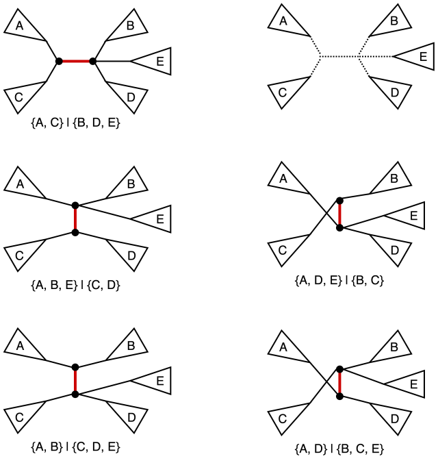
Nearest neighbor interchange (NNI) operation on a tree consists of picking an internal edge (i.e. an edge that is not incident to a leaf) deleting it along with the four edges incident to the vertices of the original edge, after obtaining four components as the result of the deletion there are three distinct ways of reconnecting them back out of which one yields the original tree. It is easy to see that for an unrooted bifurcating tree on n taxa (i.e. a tree with n leaves) there is a total of n-3 internal edges, and hence a total of 2(n-3) NNI-neighbors. We also note that the operation in this classical sense is defined for bifurcating trees (hence the guarantee that the NNI yields for connected components after the edge removal step). The figure below provides an example of NNI and the resulting tree neighbors.
The original tree is shown in the top left corner and the marked edge is the internal edge along which we perform the NNI. The four connected components labeled A, B, C, and D are shown in the top right corner. The resulting two new trees are shown at the bottom. For each of the three trees we also include the split corresponding to the marked edge.
For a small value of n we can reasonably visualize the adjacency structure on the tree space induced by the NNI operation. Namely we can identify non-isomorphic (read: distinct from the point of view of the properties we care about) labeled tree topologies as vertices and let two vertices be connected by an edge iff we can obtain one topology from another via a single NNI.
An example of adjacency graph on the space of 5 taxa unrooted bifurcating trees under the NNI operation. Original figure and caption are taken from Felsenstein, 2004, p. 40.
In general a phylogenetic tree encountered (or I guess inferred) in the wild might not be bifurcating, so it is quite natural to ask how does one generalize the notion of NNI to an arbitrary labeled unrooted tree. At the core of this operation is the process of picking a distinguished edge and then swapping components resulting from an edge deletion operation. Thus, in the case of a multifurcating tree we simply can do the same operation but with a larger set of neighbors being generated. An example is provided in the figure below.
A few possible neighbors of the original multifurcating tree (top left) under the NNI on trees with varying internal node degrees. Note that in the case where we allow multifurcations we ought to be careful in the way we define the NNI operation as some interchanges can be problematic (consider what happens if we reconnect 5 components into a star graph).
There is some amount of work on the NNI operations and NNI induced metric on phylogenetic trees (Hon and Lam, 1999), although the area tends to feel relatively sparse in terms of the research done.
Subtree prune and regraft
Subtree prune and regraft (SPR) operation on a tree consists of snipping off a branch (which can be an internal or external edge) and then inserting the snipped off subtree onto one of the edges of the remaining tree. This operation is quite well illustrated by its name, especially if you ever had to deal with grafts on actual trees (my grandfather loved to experiment with fruit tree grafting, which to his credit managed to give us a wonderful apricot half-tree on a wild apricot that used to grow in the garden). The figure below is an example of a SPR operation performed on a tree.
A subtree is snipped off from the original tree along the edge marked in red (top left) and then re-attached to the remaining tree on an edge marked in orange. It can be helpful to think of this operation as temporarily turning one of the subtrees into a rooted tree and then reinserting its root into the remaining tree.
It is easy to see that SPR operation results in a larger neighborhood set than the NNI operation. It also useful to note that any tree T’ that can be obtained from a tree T via a single NNI can also be obtained via a single SPR. In other words, if we define the set NNI(T) of trees that can be obtained from T via a single NNI, and the set SPR(T) of trees that can be obtained from T via a single SPR, then the following inclusion holds: NNI(T)⊆SPR(T) (Maddison, 1991). In the spirit of ancient geometers instead of a formalized proof, we will provide the following figure and leave it up to the reader to convince themselves that the inclusion above is indeed true.
Similarly to the NNI case we can compute the exact number of neighbors under the SPR operation for an unrooted bifurcating binary tree on n taxa. The size of this neighborhood similarly to the NNI case is independent of the topology of the tree T and is equal to 2(n-3)(2n-7) with a detailed counting argument provided by Allen and Steel, 2001 on p. 4.
We also note that the way in which we graft a subtree back in will always create an internal node of degree 3, so without a modification to this operation the question of generalizing it to multifurcating trees can be ill-posed.
Tree bisection and reconnection
Tree bisection and reconnection (TBR)operation is the most expansive operation among the three we are considering in this post, in the sense that it yields the largest neighborhoods. TBR consists of splitting the original tree T into two subtrees T’ and T” along a branch and then reconnecting them by joining any two branches of T’ and T” via an edge (in case if one of the subtrees is just a leaf the leaf is simply joined back to the tree via a new branch; in all cases vertices might have to be added to maintain a proper bifurcating tree). The figure below illustrates a TBR operation being performed.
The original tree is shown in the upper left corner. The edges to be joined are marked in orange (bottom), and the new joining edge is marked in red (bottom right). Note, that the tree obtained after the specified TBR operation is isomorphic to the tree obtained via SPR with regrafting onto the orange edge of the bottom left subtree.
The inclusion we observed for the NNI and SPR neighborhoods extends further and the following holds: NNI(T)⊆SPR(T)⊆TBR(T) (Maddison, 1991). Furthermore, by noting that any TBR can be thought of as a two step process where we first re-attach T” onto the specified edge of T’ and then reposition the attached T’ in order to get correct edge match, we can show that any TBR operation can be replicated by at most two successive SPR operations.
Finally, we note that unlike NNI and SPR, the TBR neighborhood size does depend on the topology of the tree T. However, and upper bound on the size of the neighborhood can be computed and is given by (2n-3)(n-3)2 (Allen and Steel, 2001, p.5).
Induced metrics and computational (in)tractability
We already noted in the introduction that the tree rearrangement operations induce corresponding metrics on the space of phylogenetic trees (more precisely in our current case: the space of unrooted bifurcating tree topologies). We will denote these metrics dNNI(T, T’), dSPR(T, T’), and dTBR(T, T’), respectively. From the inclusion relation on the neighborhoods it immediately follows that for any two unrooted bifurcating trees we have the following inequality: dTBR(T, T’)≤dSPR(T, T’)≤dNNI(T, T’). Furthermore, from our observation in the previous section we also can conclude that dSPR(T, T’)≤2×dTBR(T, T’).
Although we have provided an explicit example of the adjacency graph under NNI metric for the space of unrooted bifurcating trees on 5 taxa, it is not immediately obvious that in the general case the NNI adjacency graph will be connected (i.e. we are not a priori guaranteed to have a connected metric space). However, it turns out that indeed the adjacency graph under the NNI metric is indeed connected, and hence the metric space induced by dNNI(T, T’) is connected. It is easy to see that as a corollary we also get connectedness for the SPR and TBR spaces.
Since the metric spaces are connected and finite we can ask what are their respective diameters (i.e. the smallest distance between two points furthest apart in the space; this is the same definition as the graph diameter). An interesting non-trivial bound on the diameter of the NNI space was derived by Li et al., 1996: authors show that the diameter of the NNI adjacency graph (which we will denote as ΔNNI) is bounded below and above by nlogn terms. More precisely, the following inequality holds: . Allen and Steel, 2001 extend this result to the SPR and TBR cases giving the following inequalities: (a) n/2-o(n)≤ΔSPR≤n-3; (b) n/4-o(n)≤ΔTBR≤n-3.
However, knowing the diameter of a space does not imply that we can easily compute the distances within it (i.e. shortest paths via NNI, SPR or TBR operations from one tree to another). In fact, the problems of computing NNI, SPR or TBR distance between two arbitrary unrooted bifurcating trees are all NP-hard (NNI: DasGupta et al., 2000; SPR: Bordewich and Semple, 2005, Hickey et al., 2008; TBR: Hein et al., 1996). Allen and Steel, 2001 show that the SPR distance is fixed-parameter tractable, but in general the fixed-parameter tractability results in algorithms that can work efficiently only on small trees or pairs of trees which are relatively close to each other (for a more principled discussion see Whidden and Matsen, 2018). In general, it appears to be a rare case for a metric that is biologically interpretable to be efficiently computable, and vice-a-versa (take for example the Robinson-Foulds distance which is efficiently computable, but not biologically well grounded). There are some recent attempts at developing variants of tree rearrangement operations that have both biological interpretability and are computationally tractable (Collienne and Gavryushkin, 2021).
While we could possibly discuss other tree rearrangement operations or explore the discrete geometries arising from the ones we mentioned in more detail, such work would likely require multiple posts. Thus, we will wrap up here and invite the reader to continue the exploration via following the links provided in the references section.
Data and code availability
All illustrations with the exception of the one from Felsenstein, 2004 were made with draw.io. No additional materials or code were used in this post.
What’s next
I am still deliberating on the exact direction to take for the next stretch of posts, so in the meantime I am intending to continue the one-off posts where I pick a random, but interesting to me, topic in mathematical phylogeny and try to write a coherent text about it. As per usual, if you are interested in me writing about a specific topic do not hesitate to reach out.
References
Allen, Benjamin L., and Mike Steel. “Subtree transfer operations and their induced metrics on evolutionary trees.” Annals of combinatorics 5, no. 1 (2001): 1-15. https://doi.org/10.1007/s00026-001-8006-8
Bordewich, Magnus, and Charles Semple. “On the computational complexity of the rooted subtree prune and regraft distance.” Annals of combinatorics 8, no. 4 (2005): 409-423. https://doi.org/10.1007/s00026-004-0229-z
Collienne, Lena, and Alex Gavryushkin. “Computing nearest neighbour interchange distances between ranked phylogenetic trees.” Journal of Mathematical Biology 82, no. 1 (2021): 1-19. https://doi.org/10.1007/s00285-021-01567-5
Gupta, Bhaskar Das, Xin He, Tao Jiang, Ming Li, and John Tromp. “On computing the nearest neighbor interchange distance.” In Discrete Mathematical Problems with Medical Applications: DIMACS Workshop Discrete Mathematical Problems with Medical Applications, December 8-10, 1999, DIMACS Center, vol. 55, p. 125. American Mathematical Soc., 2000. PDF on author’s page
Hein, Jotun, Tao Jiang, Lusheng Wang, and Kaizhong Zhang. “On the complexity of comparing evolutionary trees.” Discrete Applied Mathematics 71, no. 1-3 (1996): 153-169. https://doi.org/10.1016/S0166-218X(96)00062-5
Hickey, Glenn, Frank Dehne, Andrew Rau-Chaplin, and Christian Blouin. “SPR distance computation for unrooted trees.” Evolutionary Bioinformatics 4 (2008): EBO-S419. https://doi.org/10.4137/EBO.S419
Hon, Wing-Kai, and Tak-Wah Lam. “Approximating the nearest neighbor interchange distance for evolutionary trees with non-uniform degrees.” In International Computing and Combinatorics Conference, pp. 61-70. Springer, Berlin, Heidelberg, 1999. https://doi.org/10.1007/3-540-48686-0_6
Li, Ming, John Tromp, and Louxin Zhang. “On the nearest neighbour interchange distance between evolutionary trees.” Journal of Theoretical Biology 182, no. 4 (1996): 463-467. https://doi.org/10.1006/jtbi.1996.0188
Maddison, David R. “The discovery and importance of multiple islands of most-parsimonious trees.” Systematic Biology 40, no. 3 (1991): 315-328. https://doi.org/10.1093/sysbio/40.3.315
Whidden, Chris, and Frederick A. Matsen. “Calculating the unrooted subtree prune-and-regraft distance.” IEEE/ACM transactions on computational biology and bioinformatics 16, no. 3 (2018): 898-911. https://doi.org/10.1109/TCBB.2018.2802911
I am currently deciding on the direction this post series will take after next week. Please check out the What’s next section and let me know if you have any preferences among described routes.
Recap
In the previous post (following Gavryushkin and Drummond, 2016) we have defined a geometry on the space of phylogenetic ultrametric trees and called the resulting metric space 𝛕-space. We also briefly mentioned the geometry on the space of trees defined by Billera, Holmes and Vogtmann, 2001, and referred to the resulting construction as BHV space.
In this post we will provide a brief overview of the algorithm presented in Owen and Provan, 2010, which allows us to compute the geodesics in 𝛕-space and BHV space in polynomial time (in the number of the tree leaves/taxa). For the ease of exposition we will delegate detailed overview of the BHV space to a later post. Hence, in what follows we will assume without the proof that BHV space is a CAT(0) complex and trees in BHV space are parametrized by the internal branch lengths with different orthants corresponding to different tree topologies.
Goal
As we mentioned before one of the key properties we want from a metric space structure on the tree space is the efficient computation of geodesics. Clearly given any finite metric space (complexes constructed in BHV or 𝛕-spaces are not finite, but the topologies are and the problem of distance within a fixed orthant determined by topology is easy to solve) we can simply consider all possible paths and then pick the one minimizing the length function. However, such approach yields an algorithm that will fail to finish computations even for modestly sized spaces.
Thus, our goal is to have an efficient algorithm that can find shortest path in polynomial time with respect to the number of leaves our trees can have.
CAT(0) properties
Since both BHV and 𝛕-spaces are CAT(0) we can leverage nice properties of the non-positively curved geometries to get an idea for an efficient algorithm. The key idea behind the algorithm comes from the following lemma (Lemma 2.1 in Owen and Provan, 2010, and Proposition 1.4, p. 160 in ).
Lemma 1.In CAT(0) space, every local geodesic is a geodesic.
Proof. Consider a local geodesic between points and . Choose a set of points such that . Note that it follows from the definition of a local geodesic that is a geodesic. Now, assume by induction that is a geodesic for all $j\leq i$. Hence, we have by the induction hypothesis and as noted above. Consider a corresponding model triangle in Euclidean space (if you forgot what a model triangle is check: Bridson and Haefliger, 2013 p. 158 or previous post on CAT spaces). Let be a point on such that . Since we are working in a CAT(0) space it follows that . On the other hand, by induction hypothesis we have . Combining this result with triangle inequality gives us , and hence and therefore . From here we can conclude that is a geodesic and hence $\Gamma_\varepsilon$ is a geodesic.
Thus, the main idea used in the paper is to start with any path between two trees (consider the path from a tree to the star tree and then back to target tree, this path called cone path is a common idea in the analyses of tree spaces; recall: Robinson-Foulds metric) and iteratively check whether it’s a local geodesic refining the path in cases when that’s not the case.
Path space geodesics
Following Owen and Provan, 2010 we will assume that the trees between which we are computing geodesics have distinct edges. We will also call two sets of edges and compatible if all pairs of splits associated with these edges are compatible, or equivalently if the union defines a tree. In other words, compatible sets of edges produce “intermediate” trees between and . Now, for a pair of partitions , of and , respectively, we can define an associated path space given that the following property holds: for every , and are compatible. To construct the path space consider the collection of orthants given by , where is the mapping of a tree to the corresponding orthant. We will call the corresponding partition pair the support, and the shortest path between and in the path space geodesic. These definitions make the geodesic in the tree space a more concrete and constructable object, which of course is important for any algorithmic approach. Furthermore, the following theorem from Billera, Holmes and Vogtmann, 2001 (see Proposition 4.1) guarantees that the path space geodesics are recovering the true geodesics.
Theorem 1. For disjoint trees the geodesic is a path space geodesic for some choice of .
We will also need the following two results, the first of which is proven in Owen, 2011 and the second in Owen and Provan, 2010 (Theorem 2.5).
Theorem 2.Let be a geodesic between and . Then there exist partitions latex \mathcal{B}=\{B_1,…,B_k\} of and , respectively, such that (a) form a support of path space in which is a path space geodesic, and (b) the following condition is satisfied:
.
A path space satisfying the above condition for its support is referred to as aproper path space, and the corresponding path space geodesic is called a proper path.
Theorem 3.A proper -path with support is a geodesic iff for each pair of edge sets in the support there is no nontrivial partition , such that is compatible with and .
Theorem 3 gives us the final ingredient needed to build out an algorithm for finding BHV space geodesics. Namely, partitions of edge sets give us a way to construct proper paths and the condition on local improvement of such proper paths guarantees that we achieve a geodesic.
Algorithm overview
As we mentioned earlier the natural choice for the starting path is the cone path between the two trees and , more formally it’s a proper path space defined by the support and the corresponding path is given by uniform contraction of all edges which results in star tree and then a follow up uniform decontraction. Now, the algorithm will proceed iteratively at each step checking whether the condition in Theorem 3 is satisfied and if not proposing a new support and a new proper path.
In order to facilitate an efficient solution for the iterative step, the problem of checking the condition of Theorem 3 and finding a new path can be recasted as an independent set problem over a bipartite graph. Namely, we will construct the incompatibility graphlatex A\subseteq E(T), B\subseteq E(T^\prime)$ as a bipartite graph with vertices given by and edges given by the pairs where the splits associated with and are incompatible. It is easy to see that for any compatibility of and is equivalent to forming an independent set in $G(E(T), E(T^\prime))$.
Thus, the condition from Theorem 3, can now be recasted as follows: Given two edge sets $A\subseteq E(T), B\subseteq E(T^\prime)$ does there exist a pair of partitions , such that the vertex set is independent in and
.
In particular, a proper path with support is geodesic iff no edge set pair satisfies the above condition.
Now, since the complement of an independent set is a vertex cover we can reformulate the above problem as a minimum weight (by transforming the inequality condition) vertex cover problem, which can be solved on bipartite graphs in . Further analysis of the algorithm steps yields that the total runtime to find the geodesic is . For the exact details of the proof of correctness of the algorithm and the runtime I suggest reading the original manuscript by Owen and Provan, 2010.
Data/code availability
This post has no associated custom code or data. Those looking for an implementation of the algorithm described should check out Megan Owen’s webpage or GitHub repo.
What’s next
This post concludes the beginning of our exploration of the geometry of the space of phylogenetic trees. There are several ways we can proceed from here.
First, we can finally start tackling the foundational paper of Billera, Holmes and Vogtmann, 2001. This path will likely require us to spend a few posts dissecting original BHV space and some associated results from metric geometry and CAT(0) spaces. We then can return to the paper of Gavryushkin and Drummond, 2016 and explore the t-space construction in a way similar to our exploration of the 𝛕-space. Finally, we can then continue our journey by catching up to more recent work by Megan Owen et al. on defining and computing statistics in BHV space (Brown and Owen, 2020), comparing phylogenetic trees with different leaf sets (Grindstaff and Owen, 2018), and extending the framework to phylogenetic cactuses (a type of phylogenetic network, Huber et al., 2021).
Second, we can instead pivot completely and ask a general question of what other geometries one can consider on the space of phylogenetic trees. In particular, we can take a look at algebraic geometry inspired view of the phylogenetic tree space as a tropical geometry (Monod et al., 2018), and an information geometry angle which gives rise to wald space (pun credit to the authors) of the phylogenetic trees (Garba et al., 2021). I will most likely skip the category theoretic angle for the topic (Baez and Otter, 2015), since frankly speaking I have no desire to introduce the notion of an operad.
Third, we can temporarily halt the process of investigating deeper into the various geometries on the tree space and ask more broadly what are geometries of interest in the case of phylogenetic networks. This route will require us to go back to some definitions of the phylogenetic network and related concepts, and will likely demand at least some amount of rehashing of the biological context.
Since, I am still debating which route is of the most interest to me at the moment, next week’s post will likely be sparser than usual, as I am figuring out which rabbit hole to pick as the next destination. However, if you actually would prefer me to pick one of these three directions do not hesitate to comment or reach out to me via other means of contact.
References
Baez, John C., and Nina Otter. “Operads and phylogenetic trees.” arXiv preprint arXiv:1512.03337 (2015). arXiv:1512.03337
Billera, Louis J., Susan P. Holmes, and Karen Vogtmann. “Geometry of the space of phylogenetic trees.” Advances in Applied Mathematics 27, no. 4 (2001): 733-767. https://doi.org/10.1006/aama.2001.0759
Bridson, Martin R., and André Haefliger. Metric spaces of non-positive curvature. Vol. 319. Springer Science & Business Media, 2013. https://doi.org/10.1007/978-3-662-12494-9
Garba, Maryam Kashia, Tom MW Nye, Jonas Lueg, and Stephan F. Huckemann. “Information geometry for phylogenetic trees.” Journal of Mathematical Biology 82, no. 3 (2021): 1-39. https://doi.org/10.1007/s00285-021-01553-x, arXiv:2003.13004
Gavryushkin, Alex, and Alexei J. Drummond. “The space of ultrametric phylogenetic trees.” Journal of theoretical biology 403 (2016): 197-208. arXiv:1410.3544
Grindstaff, Gillian, and Megan Owen. “Geometric comparison of phylogenetic trees with different leaf sets.” arXiv preprint arXiv:1807.04235 (2018). arXiv:1807.04235
Huber, Katharina T., Vincent Moulton, Megan Owen, Andreas Spillner, and Katherine St John. “The space of equidistant phylogenetic cactuses.” arXiv preprint arXiv:2111.06115 (2021). arXiv:2111.06115
Monod, Anthea, Bo Lin, Ruriko Yoshida, and Qiwen Kang. “Tropical geometry of phylogenetic tree space: a statistical perspective.” arXiv preprint arXiv:1805.12400 (2018). arXiv:1805.12400
Owen, Megan. “Computing geodesic distances in tree space.” SIAM Journal on Discrete Mathematics 25, no. 4 (2011): 1506-1529. arXiv:0903.0696
Owen, Megan, and J. Scott Provan. “A fast algorithm for computing geodesic distances in tree space.” IEEE/ACM Transactions on Computational Biology and Bioinformatics 8, no. 1 (2010): 2-13. https://doi.org/10.1109/TCBB.2010.3
In the previous post we have introduced the notion of a CAT(0) space, and briefly talked about some of the properties of CAT(0) spaces, and in particular cubical complexes. In this post, we will take this knowledge a step further into the applied direction of phylogeny. Following Gavryushkin and Drummond, 2016 we will define a metric on the space of ultrametric phylogenetic trees, show that the resulting space is CAT(0), and then discuss some of the implications of these results. Similarly to the previous post, we will have quite a bit of mathematical notation to deal with, so I will attempt to use visual aids whenever possible to improve exposition.
Motivation
One way of defining a metric on a space of phylogenetic trees is to embed the tree space into some metric space . Thus, by associating every tree in the tree space with some point in the chosen metric space, we induce a pseudometric on tree space. However, such embeddings/parameterizations are not guaranteed to be “nice” with respect to the questions we aim to answer. Namely, not all embeddings are injective (multiple distinct trees can end up being mapped to the same point in , hence in general we induce a pseudometric rather than a metric via embedding) although in the case of Gavryushkin and Drummond, 2016 the embedding has to be injective by definition. Additionally, not all embeddings are surjective (meaning that a path in might contain non-tree associated points) which creates a plethora of problems ranging from potential multiple distance minimizing solutions to the lack of tree space midpoints.
Thus, it is natural to formulate a list of desiderata for the embedding that would enable fruitful analyses. From now onwards (unless otherwise specified) we will assume that the embedding is injective.
In order to make continuous distributions behave correctly under the pullback into the tree space, we have to require the image of the embedding to be path-connected. Note, that having a path connected image is also intuitively “nice” as the continuous tree transformations would result in a path being traced out in the model metric space. Hence, we have:
(D1)The set is path-connected in .
However, being path-connected does not guarantee that the shortest path between the two points will lie within the image. Hence, we also want:
(D2) The set is convex in .
We note that the injectivity criterion forces a lower bound on the dimension of . However, if we want to define probability measure on that can be meaningfully pulled back onto we need to ensure that:
(D3) has the same dimension as .
Next, for statistical analyses to stay sound we need to ensure uniqueness of the shortest paths. This is the point in our desiderata list where you might have a brief flashback to the CAT(0) space discussion from previous week.
(D4) The space is uniquely geodesic.
Finally, since we are ultimately tackling these questions from the computer science viewpoint, we have the last desiderata that ties this into the computational realm. Namely, we want the following:
(D5) Geodesics in are computable.
In reality we probably want an even stronger version of (D5), which is:
(D5′) Geodesics in are efficiently (i.e. polynomial time) computable.
It’s worth remarking that in a general metric space we do not necessarily have (D5) with a simple example being the halting problem reduction to shortest paths in an infinite graph.
It is also important to realize that these desiderata do not guarantee existence of such embeddings, and are rather criteria for discerning more or less useful parameterizations of the tree space.
A quick aside
In general, we can attempt to parametrize the whole tree space (that’s precisely what Billera, Holmes and Vogtmann, 2001 do in their paper, which lies at the foundation of the connection between the geometry of non-positive curvature spaces and phylogenetic trees; we will refer to this space as the BHV space going forward) or we might focus on a specific subclass of trees such as ultrametric phylogenetic trees (recall that a tree is ultrametric is the distance from root to every leaf is the same). The caveat is that a parametrization that enjoys our desiderata (D1)-(D5′) for the whole tree space can fail to do so when restricted to the space of ultrametric trees. This is precisely the case for the BHV space parametrization. Hence, it can be of interest (motivated by the evolutionary models context) to explore parametrizations designed specifically for the space of the ultrametric trees. This is precisely what is done in Gavryushkin and Drummond, 2016, and what we are aiming to do in this post.
𝛕-space
We now will construct one version of a space of ultrametric trees called the 𝛕-space. To proceed consider an ultrametric tree T on n taxa, with internal nodes ordered by their time from the extant taxa. We will then parametrize the tree by mapping it to its ranked topology and a n-1-dimensional vector , where $\tau_i$ is the time difference between the i-th and i+1-th nodes. The picture below taken from Gavryushkin and Drummond, 2016 represents this parametrization for a tree on 5 taxa.
Hence, formally we have the mapping given by that embeds the space of ultrametric phylogenetic trees into a disjoint union of (Semple and Steel, 2003) non-negative real n-1-dimensional orthants (i.e. sets of the form ). We will impose an upper bound on all orthants to turn our construction into a cubical complex for the ease of the exposition. However, the construction of 𝛕-space with orthants will still yield a CAT(0) space with the key properties and desiderata (D1)-(D5′) preserved.
Note that the ranked topology in this case is a stricter condition on the shape of the tree than just the topology constraint. In particular, the two trees pictured below have distinct ranked topologies, and hence will belong to two distinct orthants in the 𝛕-space.
Figure 2. An example of two distinct ranked topologies.
Finally, to properly turn this into a cubical complex we will need to identify the isometries that glue the faces of our cubes together. However, this is rather obvious by construction, since whenever any 𝛕 coordinate becomes 0 we observe a collapse of two nodes in the ranked hierarchy to the same level. Hence, for example the two trees shown above will belong to the cubes that share the face. Since the resulting space is a cubical complex, we can naturally consider the Euclidean metric within each cube with paths for joining points in different cubes being the sums of the respective within cube paths.
The clip below shows how a tree can vary in 𝛕-space while being restricted to a single orthant determined by its ranked topology. Note that just as we discussed above in order to stay within the orthant in 𝛕-space we must keep the ranked topology constant.
For comparison, we show how a similar ultrametric tree can vary within a single fixed orthant of a BHV-space. In this case, the topology of the tree is fixed, but the ranked topology can vary.
Properties
After defining the 𝛕-space it is natural to ask whether it manages to achieve our desiderata. In order to check these properties we need to first figure out how many common faces two cubes in our complex can share (recall from the previous post that a theorem of M. Gromov gives characterization of CAT(0) cubical complexes in terms of face-sharing properties).
In general, similarly to the previous post by face of a cube we mean any sub-cube, thus it is useful to have a separate term for faces of codimension 1 (i.e. faces that are 1 less dimensional than the cubes). Hence, we will call faces of codimension 1 facets. In particular, any facet can be shared by 1, 2 or 3 cubes in total. If we let , then the resulting facet is only contained in the cube of corresponding rooted topology. If setting does not result in a multifurcating topology then the corresponding facet will be shared by exactly two cubes (see example in Figure 2 and/or Figure 2 of Gavryushkin and Drummond, 2016). Finally, if we get a multifurcation then the total number of cubes sharing the facet is 3.
Now, we are ready to take a stab at the critical result about the 𝛕-space, namely that it is a CAT(0) space, and hence uniquely geodesic. We will recall the theorem of M. Gromov here to reiterate the key result we need to prove.
Theorem 1. A cubical complex with the intrinsic Euclidean metric is CAT(0) if and only if is connected, simply connected, and for all natural : if three -cubes of share a common -cube and pairwise share common distinct -cubes, then they are contained within a -cube in .
We start by noting that the metric we introduced on our cubical complex is precisely the intrinsic Euclidean metric, and it is easy to see from our construction that the resulting complex is connected and simply connected.
To finalize the proof we need to introduce the concept of the link of a vertex v in a complex. We say that the graph G with nodes given by facets containing v and edges given by cubes that contain the two incident nodes as facets is the link of the vertex v.
First, we need to show that the cubes of the dimension (k+2) in the theorem cannot be the highest dimensional cubes in the complex. If that was the case, then the link of origin would have to contain a 3-cycle (given by the pairwise distinct (k+1)-cubes) which contradicts the result that the nearest-neighbor interchange graph does not contain 3-cycles. Thus, it follows that each of the (k+2)-cubes has at least one coordinate equal to 0. For the sake of clarity of the presentation we will assume that this is unique coordinate for each of the cubes, although the similar argument can be made in the general case. Let i, j, and r denote the respective coordinates in three cubes. We have three cases to analyze:
(i=j=r) This is impossible due to no 3-cycle property of the link of the origin.
(i=j) In this case the first two cubes must share a (k+1)-cube, and since all shared (k+1)-cubes must be pairwise distinct it cannot be the cube obtained via setting . Hence, there exists s.t. it is greater than zero in both of the first two cubes, and is zero in their shared (k+1)-cube. Now, if the first and third cube share a (k+1)-cube then it follows that their i and r coordinates both have to be zero in the shared cube, implying that the s coordinate has to be resolved in the same way between the first and third cube. However, the same exact argument can be repeated for the second and third cube implying that the first and second cubes had to be indetical.
(all distinct) In this case the left out coordinate (r for the first and second cube, i for the second and third, j for the first and third) has to be resolved the same way in the two cubes under consideration. Now, we can construct a (k+3)-cube that contains all three cubes by taking the first cube and resolving its zero coordinate (i) the same way as it is resolved in the remaining two cubes.
This analysis concludes the proof of the property required to claim that the cubical complex we defined is indeed CAT(0). It immediately follows that the geodesics in 𝛕-space are unique. At this point we are essentially done with (D1)-(D4) and the only remaining piece is the (efficient) computability of the said geodesics.
Due to the constraints on the length and scope of the post we will not dive into how does the algorithm of Owen and Provan, 2010 work in the 𝛕-space. Instead, we will discuss the algorithm in its own dedicated post.
Data and code availability
Code used to generate the 𝛕-space and BHV-space tree examples, as well as HTML outputs from Bokeh are provided in the following archive.
We spent a noticeable amount of time discussing mathematical properties of different metrics that can be imposed on tree spaces. As our next step, we will switch the lens to a computational perspective and explore the algorithm proposed by Owen and Provan, 2010. We might also touch upon more recent work in the area of the efficient computation of geodesics in CAT(0) cubical complexes. Once we are satisfied with our algorithmic solutions, we will continue the journey by exploring the BHV-space and t-space of phylogenetic trees.
References
Billera, Louis J., Susan P. Holmes, and Karen Vogtmann. “Geometry of the space of phylogenetic trees.” Advances in Applied Mathematics 27, no. 4 (2001): 733-767. https://doi.org/10.1006/aama.2001.0759
Bridson, Martin R., and André Haefliger. Metric spaces of non-positive curvature. Vol. 319. Springer Science & Business Media, 2013. https://doi.org/10.1007/978-3-662-12494-9
Gavryushkin, Alex, and Alexei J. Drummond. “The space of ultrametric phylogenetic trees.” Journal of theoretical biology 403 (2016): 197-208. arXiv:1410.3544
Owen, Megan, and J. Scott Provan. “A fast algorithm for computing geodesic distances in tree space.” IEEE/ACM Transactions on Computational Biology and Bioinformatics 8, no. 1 (2010): 2-13. https://doi.org/10.1109/TCBB.2010.3
Semple, Charles, and Mike Steel. Phylogenetics. Vol. 24. Oxford University Press on Demand, 2003.
Unlike the previous two posts it will not be obvious how what we will discuss connects to phylogeny. Furthermore, we will be diving into a noticeably more mathematically dense content this time. I will try to use some analogies and visual aids through out this post in order to make the material slightly more accessible.
Introduction
Geometry is a wonderful subject (even if I struggled with it in high school) that makes appearances in many aspects of various sciences (including social ones). However, musing about geometry at large is better left to people who are (a) more proficient in the study of it, and (b) have an acumen for writing more lengthy works, hence I will simply point you in the direction of Jordan Ellenberg’sShape. What we will concern ourselves with today is a more specific slice of the geometry in which we will look at metric spaces of non-positive curvature. I will not define the notion of a metric space again, as you can simply navigate either to the previous post in the series or Wikipedia. The bulk of this post will consist of defining non-positive curvature, and then we will follow up with a few properties of such spaces, and some examples.
Geodesics are a natural notion extending the concept of the “shortest” path curve to general metric space framework. More precisely, given a metric space a geodesic from to is the map s.t. and . We will call a metric space a geodesic space if for any there exists a geodesic from to . Furthermore, if for all pairs of points such geodesic is unique we will call such space uniquely geodesic (see Bridson and Haefliger, 2013, pp. 4-8 for additional details and examples).
For example, the classic Euclidean space is uniquely geodesic with the geodesics given by straight lines, i.e. for any two points we have the geodesic given by . On a sphere geodesic between two points is the arc segment obtained by intersecting a plane through , and the center of the sphere with the surface (i.e. the great circle arc). An example of a geodesic triangle on a sphere is given below (image courtesy of Wikipedia).
Note, that a sphere is not a uniquely geodesic space, since any pair of diametrically opposed points has an infinite set of possible geodesics between them.
Triangles
Just like the notion of a geodesic extends our naïve understanding of the shortest paths, the notion of a geodesic triangle (Bridson and Haefliger, 2013, p. 158) extends our notion of a triangle. Given a metric space a geodesic triangle is a set of tree points called vertices and a choice of three geodesic segments joining them called sides, we will denote such a triangle or more briefly . Note, that the later notation is not precise, as in the case of a non-uniquely geodesic space there is not necessarily a unique choice of a geodesic between two vertices. Finally, we will write to indicate that belongs to the union .
In order to define a CAT(k) space we also need the notion of a comparison triangle. In order to avoid a lengthy (and somewhat involved) discussion of the nuances about the model spaces and corresponding notation, we will focus on three general types of model spaces: Euclidean n-dimensional space, the n-sphere, and hyperbolic n-space. We already defined geodesics in the case of . For the n-sphere we will define the metric via cosine distance where the inner product is in the corresponding embedding and the corresponding geodesics are given by minimal great arcs (for full definition and description see Bridson and Haefliger, 2013, pp. 16-17). For the hyperbolic n-space we will use the same construction as Bridson and Haefliger, 2013 (p. 18-20) by considering the space which consists of with bilinear form and defining . The distance on this space will be given by (similarly to the sphere case, see Bridson and Haefliger, 2013, pp. 18-23 for details).
Finally, a comparison triangle is a triangle in the model space that satisfies , , and . A point for is called a comparison point if . Note, that for we need an additional condition on the perimeter of a triangle to guarantee existence of a comparison triangle, for the purposes of this post we will state the condition, but not elaborate on it in detail.
CAT(k)
So what’s a cat? It’s a gorgeous animal that many humans have as a pet. Many cats are fluffy, and so is mine. Also cats are silly and generally cool to have around. However, this post is not about these kinds of cats.
The term “CAT(k)” space was coined by Mikhail Gromov and consists of three initials honoring: Élie Cartan, Alexander D. Alexandrov, and Victor A. Toponogov. Now, we will define a CAT(k) space. Let be a metric space and let be a real number. Let be a geodesic triangle in with perimeter less than (the diameter of the space, this is the condition need to guarantee the existence of comparison triangle). Then we say that satisfies the CAT(k) inequality if for the corresponding comparison triangle and all with corresponding comparison points the inequality is satisfied. Thus, for a we will call a CAT(k) space if is geodesic and all its geodesic triangles satisfy the CAT(k) inequality. For , we relax definition by only requiring to be -geodesic and only requiring the inequality condition for triangles of perimeter bounded by .
Finally, we will call a space to be of curvature at most if it is locally a CAT(k) space. Hence, any space that is (locally) CAT(0) is a space on non-positive curvature (in the Alexandrov sense).
Intuitively speaking the triangles in a CAT(k) space have to be thinner than the ones in the corresponding model space. In particular, triangles in CAT(0) spaces are thinner than those in the regular Euclidean space (namely given two points on the sides of a triangle the distance between them in CAT(0) space is less than or equal to the distance between the corresponding comparison points in the Euclidean space). The illustration below shows three model spaces (sphere, plane, and hyperbolical paraboloid) and a cat drawn in each space. You can see that sphere cat is chubbier than the flat cat, which is chubbier than the hyperbolic cat, turns out triangles in these spaces are also of different chubbiness.
For the rest of the post we will focus specifically on the case of the CAT(0) spaces, as they present the most interest to us in the follow up posts.
An immediate, but important consequence of the definition of a CAT(k) space is that any CAT(0) space is uniquely geodesic. Note, that being uniquely geodesic also implies that a space is contractible (the converse does not hold, there are contractible spaces that are not uniquely geodesic, a simple example is the closed upper hemisphere which is clearly contractible, and also not uniquely geodesic for the same reason a sphere isn’t).
Next, we will briefly describe some interesting spaces which under certain conditions turn out to be CAT(0).
My CAT is a cubical complex!
Let be the unit interval, then we call the n-fold product the unit cube. We will let denote a point by convention. Since we will be mainly operating in dimensions, we will use the term “face” to describe any-dimensional face of the cube. Thus, the faces of are $\{0\}, \{1\}$ (the 0-dimensional faces), and (the 1-dimensional face). Analogously, for a faceis a subset which can be written as where each is a face of . The dimension of the face will be the sum of dimensions of , and we also note that a k-dimensional face will be isometric to .
Now, we are ready to define a cubical complex (Def. 7.32 from Bridson and Haefliger, 2013) in a similar vein to the definition of a simplicial complex (for those familiar with the latter construction). A cubical complex is the quotient of a disjoint union of cubes by an equivalence relation with the restrictions of the natural projection satisfying
for every the map is injective;
if then there is an isometry from a face onto a face such that .
While not precisely a cubical complex, the above rendition of a cat is reminiscent of one. The picture was taken from: https://www.boredpanda.com/i-made-animal-cube. All credit for creating those goes to the original author(s), which as far I found is: Aditya Aryanto.
Note, that in general a cubical complex needs not be a CAT(0) space. However, the following theorem of Gromov, 1987 gives the necessary and sufficient conditions for a cubical complex to be CAT(0).
Theorem 1. A cubical complex with the intrinsic Euclidean metric is CAT(0) if and only if is connected, simply connected, and for all natural : if three -cubes of share a common -cube and pairwise share common distinct -cubes, then they are contained within a -cube in .
A bit of perspective
In many cases the underlying geometry of the solution space can make or break our ability to solve problems efficiently. For example, many interesting discrete problems are NP-hard, and often do not even have good approximations (for a deeper dive Google “inapproximability results”, Khot, 2010 gives a great overview). In general, computing geodesics is a hard problem, but in certain spaces we can still efficiently compute (meaning in polynomial time) or approximate geodesics. CAT(0) cubical complexes are one particular class of “nice” spaces, meaning that geodesics can be computed or approximated well enough in polynomial time (Owen, and Provan, 2010, Hayashi, 2021). Implications of these algorithmic results mean that in certain phylogenetic (and robotics) problems we are able to efficiently compute distance between two points in the space, and reconstruct the optimal path between them (or at least do so up to error).
Code and data availability
All code used in this post is available in the following Jupyter notebook.
The next post in the series will take us back to the world of phylogeny, but this time armed with the knowledge about CAT(0) spaces. We will try to make sense of defining nice metrics on the space of phylogenetic trees with branch lengths, and learn a thing or two in the process. Essentially, the idea for the remainder of this stretch of the series will be to work our way through the paper of Gavryushkin and Drummond, 2016 on the space of ultrametric phylogenetic trees.
References
Bridson, Martin R., and André Haefliger. Metric spaces of non-positive curvature. Vol. 319. Springer Science & Business Media, 2013. https://doi.org/10.1007/978-3-662-12494-9
Gavryushkin, Alex, and Alexei J. Drummond. “The space of ultrametric phylogenetic trees.” Journal of theoretical biology 403 (2016): 197-208. arXiv:1410.3544
Hayashi, Koyo. “A polynomial time algorithm to compute geodesics in CAT (0) cubical complexes.” Discrete & Computational Geometry 65, no. 3 (2021): 636-654. arXiv:1710.09932
Khot, Subhash. “Inapproximability of NP-complete problems, discrete Fourier analysis, and geometry.” In Proceedings of the International Congress of Mathematicians 2010 (ICM 2010) (In 4 Volumes) Vol. I: Plenary Lectures and Ceremonies Vols. II–IV: Invited Lectures, pp. 2676-2697. 2010. https://cs.nyu.edu/~khot/papers/icm-khot.pdf
Owen, Megan, and J. Scott Provan. “A fast algorithm for computing geodesic distances in tree space.” IEEE/ACM Transactions on Computational Biology and Bioinformatics 8, no. 1 (2010): 2-13. https://doi.org/10.1109/TCBB.2010.3
Since my blog has been experiencing a shortage of content (mostly due to the fact that I am busy with my current research work), I decided to try out a new format that will hopefully motivate me to post more often. “Weekies” i.e. “weekly quickies” are going to be weekly posts of small puzzles that I come up with or come across on the web. I plan to follow up each “weeky” with a longer write-up of solution and discussion roughly within a month or so of the original post. In the meantime do not hesitate to post solutions and discuss the puzzle in the comments under the original post.
Random walks
Consider the K4 graph/tetrahedron depicted below. The following questions concern different random walks starting at the vertex A.
Q1. Assume that at any time step we will move to a random neighboring vertex with the equal probability of 1/3. What’s the probability that we will visit all vertices of the graph before returning to A?
Q2. Given the same walk as in question 1, what’s the probability that we will visit any one vertex out of {B, C, D} at least n times before returning to A?
Q3. Now, let’s change our walk to have a 1/2 probability of remaining at the current vertex and probabilities of 1/6 to move to each of the neighboring vertices. How do answers to questions 1 and 2 change for this walk?
Q4. With the walk described in question 3, what is the expected number of steps we need to take to visit all vertices at least once?
Q5. Let us record the sequence of visited vertices as a string of characters A, B, C, D. Consider a random walk in question 3 and record its first 10 vertices. What’s the probability that the string “ABCD” occurs as a subsequence in the recorded sequence?
Q6. We can generalize the walk described in question 3 using the parameter q ∈ [0, 1] by letting the probability of staying at the current vertex be q and probability of going to any given neighbor be (1-q)/3. Additionally, let the start vertex be picked uniformly at random. Let n be the length of the sequence of vertices that we record, analogously to question 5. Let Pq,n be the distribution on the Ω={A, B, C, D}n generated by the described process. Let Un be the uniform probability distribution on the Ω. Let D be the total variation distance function and let us denote d(q,n) = D(Pq,n, Un). Investigate behavior of the function d : [0, 1] ⨉ ℕ → [0, 1].
I was sitting in my office, a couple of weeks ago, minding my regular bioinformatics flavored business with a cup of oolong tea, when Senthil stopped by and told me that he has a puzzle he’d like some help with. Now, both me and Senthil enjoy math and we especially enjoy small nifty tricky problems. Thus, the puzzle he shared was the following.
Consider a unit grid on a plane. Pick a non-negative real number L. Now, we can place a random segment of length L in the plane by picking a point and an angle uniform at random and drawing a segment of length L originating at the chosen point and oriented based on the chosen angle. Which value of L maximizes the probability that this segment will intersect exactly one line of the grid?
We spent about 5 minutes chatting about different placements of the segment, probabilities, and our lack of desire to compute a nasty triple integrals. We had to wrap up quickly since, I was short on time and had to finish up some other tasks.
Last Thursday I was co-organizing our department’s happy hour, and Senthil reminded me of the outstanding problem. I made a pinky promise that I’ll help on Friday, which brings us to the story I am about to tell you.
Do not integrate, just simulate!
Since, I was not sold on the idea of computing integrals first thing on a Friday morning, I decided to quickly write up a simulation that would do exactly what the problem statement described. After about 20 minutes of typing away, I had my tiny C program up and running and spitting out probabilities with 6 sweet significant digits. Senthil came by quite soon, and within 40 minutes of back and forth of computer assisted linear search we were quite certain our answer for L was 1. Yay, problem solved, L = 1, probability is approximately 0.63774, and we can all go drink coffee and do whatever Computer Science PhD students do on a Friday. Well, no.
Of course we were not happy, I meant what is 0.63774? Have you heard of this number before? Does it have any meaning? Is this the number of goats you must sacrifice to Belial before you learn the great mysteries of the world? We took to OEIS and found (among other amazing things) that 0, 6, 3, 7, 7 is a subsequence in the decimal expansion of Mill’s constant, assuming the Riemann hypothesis is true. Other than that the number didn’t quite give us an immediate answer. We also checked the magic of WolframAlpha, which gave us some neat ideas, like (3 π)/(2 e^2). However, as you can guess reverse engineering this fraction was 1) stupid; 2) hard; and finally 3) something we didn’t do.
In the meantime, we decided to put our theory hats back on and figure out what is happening, and how we can get an analytical expression of this probability. Senthil recalled that in fact there is a very similar well-known question, called Buffon’s needle problem, which has an amazingly clean solution. However, we could not see how one can easily translate the setting of that problem to ours. After some amount of drawing, complaining about integrals and debating which events are measure zero, we decided to take a coffee break and walk outside for a bit. This is when the major theoretical breakthrough happened.
Senthil noticed that instead of thinking about the grid as a whole, we can consider two sets of parallel lines independently. The advantage of this view was clear, now we have the Buffon’s needle problem embedded into ours directly! We multiplied some probabilities, got wrong numbers and complained about futility of theoretical efforts. Then we of course reimagined how stuff should be multiplied and counted things again, and again, and again. Are the events independent? Do we count this in or subtract it out? Do we go back to the integral formula?
Clearly the two intersection events are not independent, since the orientation (based on angle) that works well for horizontal intersection, is not favorable for the vertical one. Thus we can’t just multiply stuff out and subtract from one. Thus, we went back to the integral. This is where things got tangled up. We recomputed the triple integral a few times, but something was not tying out. We computed integral of a product of integrals and something still didn’t tie out. We have been running in circles, seeing numbers like 0.202 and 0.464 all over the place. Finally, the original answer to Buffon’s needle, the 2/π, was temptingly close to our own, since it was 0.636619. Finally, around 4pm we threw in the towel and parted ways.
Simulation clearly saved the day, and even if we were not sure of the theory behind this number, we knew the answer with high confidence, and that was already a win. But…
Back to the drawing and integration
I took out a piece of paper, folded it in four, and started sketching. There is a nice video out there that explains how to derive solution to the Buffon’s needle problem. Thus, I just went through the steps, drawing out the circle, and thinking what are the exact conditions we need to satisfy to get our segment intersect exactly one grid line.
The shaded region above represents the range of admissible positions for the needle (black arrow) when the angle formed by needle and x-axis does not exceed 90 degrees. Note that we only consider intersection with the line , since the intersection with the line is identical by symmetry.
Now, considering the angle of the needle to x-axis to be and distances to horizontal and vertical lines to be and respectively, we can define the conditions for the admissible position as . Thus, we can write down our desired integral, and evaluate it as . Now, dividing through by the total area and multiplying by 2, due to symmetry for the intersection to the second line, we arrive at the coveted . Case can be rested, we now have a neat theoretical solution to the question, and a beautiful mathematical expression as an answer. However, I am still unhappy, because I cannot ascribe the error we see in the simulation to pure numerical precision at this scale.
The devil is in the details: wording and measure zero events
One of the first things you learn in a probability theory class is that events of measure zero don’t matter. Picking a specific point on a line, or even picking a rational point on a line are measure zero events, hence they don’t really matter when you calculate probabilities. Nevertheless simulations are not only countable, they are finite! Which means accidentally dropping in an event of measure zero that shouldn’t be there can trip you up. This is exactly what happened in our case. We want to count the number of times a random segment intersects exactly one line of the grid. Now, I assumed this condition meant instead: segment intersects the grid at exactly one point! The difference shines for the points that are intersections of the two sets of parallel lines forming the grid, because they are a single grid point, but a segment crossing this point in fact intersects not one, but two lines!
I have adjusted my counting scheme to correctly reflect this edge case as intersecting two lines, and therefore, not being a favorable outcome. Guess what happened next… Exactly, the sweet shiny 0.6366313 popped out of my simulation as the predicted probability of the event. Of course, this number is closer to than our previous candidate, and now all the doubts are gone, the theory and simulation agree!
Discussion and lessons learned
First of all, if my simulation runs in about 2 minutes (going through 500,000,000 random segments), why not run a longer simulation to counter the effect of nasty accidental event? Well, numbers have their limits on computers, and overflows happen. I tried running the simulation for 2,000,000,000 and 20,000,000,000 segments. The first run gave a slightly smaller number than the original 0.6377, but still not quite 0.6366. The second one, gave a whooping probability of -8.648, which even those not too familiar with measure theoretic probability would call out as absurd. Can I spend more time bugfixing this, and get a great simulator, that can scale to 1,000,000,000,000 segment trial? Yes. Is it reasonable to pour time into this? No!
Second, why not do the theory neatly from the start? At the end of the day the problem really takes about 30 minutes of careful drawing and setup and 3 minutes of WolframAlpha-ing the integral. Well, first this involves dissecting the problem theoretically which takes time. Second, writing up the simulator took 20 minutes, for contrast understanding how the Buffon’s needle problem is solved took about the same 15-20 minutes. The latter on its own didn’t give a solution, the former at least provided a good numerical estimate. Finally, recall how the problem is actually about finding the optimal length L? Well, that was quite a block to developing nice theoretical answer, once we were quite certain L is 1, we could actually focus on the theory that mattered.
Third, why not read the problem statement carefully and not jump to wild assumptions? Well, this one goes into lessons learned bucket, alongside the entire finiteness of simulations shenanigans. You would expect that years of problem solving would teach me that, and yet again, I make the same mistakes.
Overall I can say that this was an amazing exercise in basic probability, geometry and mocking up simulations to solve puzzle problems. I am happy to learn that writing a quick program can help in figuring out theory behind a question. Furthermore, I am also quite delighted to experience nuances of probability first hand, without putting important questions and results on the line.
Final notes and resources
Many thanks to Senthil Rajasekaran for bringing this problem to my attention and guiding me through the crucial steps on getting the theoretical answer in the scopes. Looking forward to more puzzles to solve!
My code for the simulator is available in this (zipped) file. Note that the random number generator was lifted from a course by Benoit Roux at UChicago, and the rest of the code is mine. The commented out portion of the intersect function is exactly what caused the annoying of by 0.0011 error.
Thanks for the attention, and happy bug catching y’all!


![[n]=\{1, 2, 3, ..., n\}](https://s0.wp.com/latex.php?latex=%5Bn%5D%3D%5C%7B1%2C+2%2C+3%2C+...%2C+n%5C%7D&bg=fafafa&fg=6c6c8c&s=0&c=20201002)
![f:[n]\to[n]](https://s0.wp.com/latex.php?latex=f%3A%5Bn%5D%5Cto%5Bn%5D&bg=fafafa&fg=6c6c8c&s=0&c=20201002)
![\mathcal{F}_n=\{f|f:[n]\to[n]\}](https://s0.wp.com/latex.php?latex=%5Cmathcal%7BF%7D_n%3D%5C%7Bf%7Cf%3A%5Bn%5D%5Cto%5Bn%5D%5C%7D&bg=fafafa&fg=6c6c8c&s=0&c=20201002)

![i\in[n]](https://s0.wp.com/latex.php?latex=i%5Cin%5Bn%5D&bg=fafafa&fg=6c6c8c&s=0&c=20201002)


![j\in[n]](https://s0.wp.com/latex.php?latex=j%5Cin%5Bn%5D&bg=fafafa&fg=6c6c8c&s=0&c=20201002)


![[n]](https://s0.wp.com/latex.php?latex=%5Bn%5D&bg=fafafa&fg=6c6c8c&s=0&c=20201002)


![\sigma:[n]\to[n]](https://s0.wp.com/latex.php?latex=%5Csigma%3A%5Bn%5D%5Cto%5Bn%5D&bg=fafafa&fg=6c6c8c&s=0&c=20201002)


![\mathbb{E}[X]=\sum_{\sigma}\mathbb{E}[X_\sigma]=\sum_{\sigma}Pr(X_\sigma =1)](https://s0.wp.com/latex.php?latex=%5Cmathbb%7BE%7D%5BX%5D%3D%5Csum_%7B%5Csigma%7D%5Cmathbb%7BE%7D%5BX_%5Csigma%5D%3D%5Csum_%7B%5Csigma%7DPr%28X_%5Csigma+%3D1%29&bg=fafafa&fg=6c6c8c&s=0&c=20201002)
![\mathbb{E}[X]=(n-1)!/2^n](https://s0.wp.com/latex.php?latex=%5Cmathbb%7BE%7D%5BX%5D%3D%28n-1%29%21%2F2%5En&bg=fafafa&fg=6c6c8c&s=0&c=20201002)


 .
.  between points
  and
and  . Choose a set of points
  such that
  . Note that it follows from the definition of a local geodesic that
  is a geodesic. Now, assume by induction that
  is a geodesic for all $j\leq i$. Hence, we have
  by the induction hypothesis and
  as noted above. Consider a corresponding model triangle
  in Euclidean space (if you forgot what a model triangle is check:
  be a point on
  such that
  . Since we are working in a CAT(0) space it follows that
  . On the other hand, by induction hypothesis we have
  . Combining this result with triangle inequality gives us
  , and hence
  and therefore
  . From here we can conclude that
  is a geodesic and hence $\Gamma_\varepsilon$ is a geodesic.
 between which we are computing geodesics have distinct edges. We will also call two sets of edges
  and
and  compatible if all pairs of splits associated with these edges are compatible, or equivalently if the union
  defines a tree. In other words, compatible sets of edges produce “intermediate” trees between
  and
and  . Now, for a pair of partitions
  ,
,  of
of  and
and  , respectively, we can define an associated path space given that the following property holds: for every
  ,
,  and
and  are compatible. To construct the path space consider the collection of orthants
  given by
  , where
  is the mapping of a tree to the corresponding orthant. We will call the corresponding partition pair
  the support, and the shortest path between
  the path space geodesic. These definitions make the geodesic in the tree space a more concrete and constructable object, which of course is important for any algorithmic approach. Furthermore, the following theorem from
  .
. be a geodesic between
  latex \mathcal{B}=\{B_1,…,B_k\} of
  .
. -path
-path  in the support there is no nontrivial partition
  ,
,  such that
  is compatible with
  and
and  .
. and the corresponding path is given by uniform contraction of all edges which results in star tree and then a follow up uniform decontraction. Now, the algorithm will proceed iteratively at each step checking whether the condition in Theorem 3 is satisfied and if not proposing a new support and a new proper path.
  latex A\subseteq E(T), B\subseteq E(T^\prime)$ as a bipartite graph with vertices given by
  where the splits associated with
  and
and  are incompatible. It is easy to see that for any
  compatibility of
  and
and  is equivalent to
  ,
,  such that the vertex set
  is independent in
  and
and  satisfies the above condition.
 . Further analysis of the algorithm steps yields that the total runtime to find the geodesic is
  . For the exact details of the proof of correctness of the algorithm and the runtime I suggest reading the original manuscript by
  into some metric space
  . Thus, by associating every tree in the tree space with some point in the chosen metric space, we induce a pseudometric on tree space. However, such embeddings/parameterizations are not guaranteed to be “nice” with respect to the questions we aim to answer. Namely, not all embeddings are injective (multiple distinct trees can end up being mapped to the same point in
  , hence in general we induce a pseudometric rather than a metric via embedding) although in the case of
  that would enable fruitful analyses. From now onwards (unless otherwise specified) we will assume that the embedding
  is injective.
  is path-connected in
  , where $\tau_i$ is the time difference between the i-th and i+1-th nodes. The picture below taken from
 that embeds the space of ultrametric phylogenetic trees into a disjoint union of
  (
( ). We will impose an upper bound on all orthants to turn our construction into a cubical complex for the ease of the exposition. However, the construction of 𝛕-space with orthants will still yield a CAT(0) space with the key properties and desiderata (D1)-(D5′) preserved.
 face. Since the resulting space is a cubical complex, we can naturally consider the Euclidean metric within each cube with paths for joining points in different cubes being the sums of the respective within cube paths.
 , then the resulting facet is only contained in the cube of corresponding rooted topology. If setting
  does not result in a multifurcating topology then the corresponding facet will be shared by exactly two cubes (see example in Figure 2 and/or Figure 2 of
  with the intrinsic Euclidean metric is CAT(0) if and only if
  : if three
  -cubes of
  -cubes, then they are contained within a
  -cube in
  . Hence, there exists
  s.t. it is greater than zero in both of the first two cubes, and is zero in their shared (k+1)-cube. Now, if the first and third cube share a (k+1)-cube then it follows that their i and r coordinates both have to be zero in the shared cube, implying that the s coordinate has to be resolved in the same way between the first and third cube. However, the same exact argument can be repeated for the second and third cube implying that the first and second cubes had to be indetical.
 a geodesic from
  is the map
 ![c:[0, l]\to X](https://s0.wp.com/latex.php?latex=c%3A%5B0%2C+l%5D%5Cto+X&bg=fafafa&fg=6c6c8c&s=0&c=20201002) s.t.
s.t.  and
and  . We will call a metric space a geodesic space if for any
  there exists a geodesic from
  we have the geodesic given by
  . On a sphere geodesic between two points
  is the arc segment obtained by intersecting a plane through
 is a set of tree points
  called vertices and a choice of three geodesic segments
 ![[p, q], [q, r], [r, p]](https://s0.wp.com/latex.php?latex=%5Bp%2C+q%5D%2C+%5Bq%2C+r%5D%2C+%5Br%2C+p%5D&bg=fafafa&fg=6c6c8c&s=0&c=20201002) joining them called sides, we will denote such a triangle
joining them called sides, we will denote such a triangle ![\Delta([p, q], [q, r], [r, p])](https://s0.wp.com/latex.php?latex=%5CDelta%28%5Bp%2C+q%5D%2C+%5Bq%2C+r%5D%2C+%5Br%2C+p%5D%29&bg=fafafa&fg=6c6c8c&s=0&c=20201002) or more briefly
or more briefly  . Note, that the later notation is not precise, as in the case of a non-uniquely geodesic space there is not necessarily a unique choice of a geodesic between two vertices. Finally, we will write
  to indicate that
 ![[p, q]\cup [q, r]\cup [r, p]](https://s0.wp.com/latex.php?latex=%5Bp%2C+q%5D%5Ccup+%5Bq%2C+r%5D%5Ccup+%5Br%2C+p%5D&bg=fafafa&fg=6c6c8c&s=0&c=20201002) .
.  Euclidean n-dimensional space,
  the n-sphere, and
  hyperbolic n-space. We already defined geodesics in the case of
  . For the n-sphere we will define the metric via cosine distance
  where the inner product is in the corresponding embedding
  and the corresponding geodesics are given by minimal great arcs (for full definition and description see
  which consists of
  with bilinear form
  and defining
  . The distance on this space will be given by
  (similarly to the sphere case, see
  is a triangle in the model space
  that satisfies
  ,
,  , and
, and  . A point
 ![\overline{x}\in[\overline{p}, \overline{q}]](https://s0.wp.com/latex.php?latex=%5Coverline%7Bx%7D%5Cin%5B%5Coverline%7Bp%7D%2C+%5Coverline%7Bq%7D%5D&bg=fafafa&fg=6c6c8c&s=0&c=20201002) for
for ![x\in[p, q]](https://s0.wp.com/latex.php?latex=x%5Cin%5Bp%2C+q%5D&bg=fafafa&fg=6c6c8c&s=0&c=20201002) is called a comparison point if
is called a comparison point if  . Note, that for
  we need an additional condition on the perimeter of a triangle to guarantee existence of a comparison triangle, for the purposes of this post we will state the condition, but not elaborate on it in detail.
  (the diameter of the
  satisfies the CAT(k) inequality if for the corresponding comparison triangle
  and all
  with corresponding comparison points
  the inequality
  is satisfied. Thus, for a
  we will call
  -geodesic and only requiring the inequality condition for triangles of perimeter bounded by
![I=[0, 1]](https://s0.wp.com/latex.php?latex=I%3D%5B0%2C+1%5D&bg=fafafa&fg=6c6c8c&s=0&c=20201002) be the unit interval, then we call the n-fold product
be the unit interval, then we call the n-fold product  the unit cube. We will let
  denote a point by convention. Since we will be mainly operating in
 ![[0, 1]](https://s0.wp.com/latex.php?latex=%5B0%2C+1%5D&bg=fafafa&fg=6c6c8c&s=0&c=20201002) (the 1-dimensional face). Analogously, for
(the 1-dimensional face). Analogously, for  which can be written as
  where each
  is a face of
  . The dimension of the face will be the sum of dimensions of
  .
.  by an equivalence relation
  with the restrictions
  of the natural projection
  satisfying
 the map
  is injective;
 then there is an isometry
  from a face
  onto a face
  such that
  .
.
 error).

 , since the intersection with the line
  is identical by symmetry.
 and distances to horizontal and vertical lines to be
  and
and  respectively, we can define the conditions for the admissible position as
  . Thus, we can write down our desired integral, and evaluate it as
  . Now, dividing through by the total area and multiplying by 2, due to symmetry for the intersection to the second line, we arrive at the coveted
  . Case can be rested, we now have a neat theoretical solution to the question, and a beautiful mathematical expression as an answer. However, I am still unhappy, because I cannot ascribe the error we see in the simulation to pure numerical precision at this scale.
 than our previous candidate, and now all the doubts are gone, the theory and simulation agree!